I have already given an argument for the non-consonance of the Sorgenfrey line Rℓ here. As I have said last time, I would like to deal with the case of the space Q of rational numbers, and explain an argument due to Costantini and Watson [4]. Before we start, let me make an apology. This is probably the longest post I will ever have made, and it is pretty technical, too. Nonetheless, I have made my best to make the argument readable. Please forgive me if you find that all that is too long!
A bit of history
That Q is not consonant was first proved by A. Bouziad [2]. His argument is a pretty simple measure theoretic argument, which shows that every consonant space is a Prohorov space, namely a space X such that the compact subsets of P(X) are exactly the uniformly tight sets—P(X) is the space of Radon probability measures on X, with the weak topology. As you may have guessed, this requires some knowledge of topological measure theory, which I will not get into. But this is not so difficult to acquire. The real difficulty is the second step: you need to argue that Q is not a Prohorov space, and that is a deep and technically demanding result due to D. Preiss [3].
Another argument was proposed by C. Costantini and S. Watson [4] a few years later. This one is much easier to explain. It is an elementary argument, one which builds fairly strange objects, but at least one that one can describe explicitly. Note that by elementary, I mean an argument that does not require elaborate notions or a lot of prior knowledge; an elementary argument need not be simple.
Consonant spaces
As promised, let me recall that what a consonant space is. I have already spoken about them, for example here, here, or much more recently, here, but I guess that a refresher is never inappropriate.
Given any topological space X, you can form its lattice of open sets OX, and then consider it with the Scott topology of inclusion. Among the Scott-open subsets of OX, you can find the sets of the form ■Q, where Q is compact saturated in X: ■Q is the collection of open neighborhoods of Q, and the fact that Q is compact entails that ■Q is Scott-open in OX. In fact, if X is sober, those sets ■Q are the only Scott-open filters that exist, by the Hofmann-Mislove theorem (Theorem 8.3.2 in the book). Any union of sets of the form ■Q is Scott-open in OX, but does the converse hold? A space X is consonant precisely when this is the case, namely precisely when every Scott-open subset of OX is a union of sets of the form ■Q with Q compact saturated.
The notion, introduced in [1], crops up regularly.
The consonant spaces are exactly those spaces X such that the Isbell and compact-open topologies coincide, on any space of continuous maps from X to any topological space Y (or just for Y=S, the Sierpiński space).
Every locally compact space is consonant (Exercise 5.4.12), and every T3 Čech-complete space is consonant (Exercise 8.3.4, namely the Dolecki-Greco-Lechicki theorem: Theorem 4.1 in [1]). Hence in particular Baire space NN is consonant, although it is not locally compact. Since then, we have learned that all quasi-Polish spaces, and even all LCS-complete spaces are consonant [5, Proposition 12.1].
In an important paper [6], M. de Brecht and T. Kawai have considered the question of the commutativity between the Hoare and Smyth hyperspace constructions. (It had been well known that the Hoare and Smyth powerlocales commute [7], without any assumption. But power locales and hyperspaces do not always coincide.) Let me not describe the question fully, and let me remain elusive about a few details. There is a Hoare hyperspace H(X) consisting of the closed subsets of X, with the so-called lower Vietoris topology. There is also a Smyth hyperspace Q(X) consisting of the compact saturated subsets of X, with the upper Vietoris topology. Now there is a continuous map σ : H(Q(X)) → Q(H(X)), which maps every closed subset C of Q(X) to {C ∈ H(X) | C intersects every compact subset of X that is in C}. De Brecht and Kawai show that σ is a homeomorphism if and only if X is consonant.
All right! Let us start attacking the question of the failure of consonance of Q for good.
Q is zero-dimensional
Q, as a subspace of R, is second-countable. Contrarily to R, it is zero-dimensional, meaning that its topology has a base of clopen sets. (A set is clopen if and only if it is both open and closed.)
Explicitly, for every irrational number z, the set Q ∩ ]–∞, z[ is open. Its complement in Q is the set Q ∩ ]z, +∞[, since z is irrational, and that complement is open, too. Hence both Q ∩ ]–∞, z[ and Q ∩ ]z, +∞[ are clopen. It follows that, for any two irrational numbers z<z’, Q ∩ ]z, z’[ is also clopen, as the intersection of Q ∩ ]–∞, z’[ and of Q ∩ ]z, +∞[. Now, given any point x of Q and any open neighborhood Q ∩ U of x in Q (where U is open in R), U contains an open interval ]a, b[ that contains x, and then there are irrational numbers z and z’ such that a<z<x and x<z’<b. Hence the clopen set Q ∩ ]z, z’[ is an open neighborhood of x included in Q ∩ U. This shows that the sets Q ∩ ]z, z’[ with z<z’ irrational form a base of clopen sets.
This base is uncountable, but there must be a countable one, by the following observation, and the fact that Q is second-countable (its topology is generated by sets Q ∩ ]a, b[ where a<b are both rational).
Lemma A. Every second-countable, zero-dimensional space has a countable base of clopen sets.
Proof. Let Vn, n ∈ N, enumerate the elements of a given countable base of the topology of a second-countable, zero-dimensional space X. Let me say that the pair of natural numbers (m, n) is good if and only if not only Vm is included in Vn, but there is even a clopen set O such that Vm ⊆ O ⊆ Vn. For every good pair (m, n), we pick exactly one clopen set Omn such that Vm ⊆ Omn ⊆ Vn. (Yes, we use to axiom of (countable) choice to do so.) I claim that the sets Omn form a countable base of clopen sets.
To this end, it suffices to show that they form a base. Let x be any point of X, and U be any open neighborhood of x in X. Since the sets Vn form a base of the topology, we can find one such that x ∈ Vn ⊆ U. Since X is zero-dimensional, there is a clopen set O such that x ∈ O ⊆ Vn. Since the sets Vm, m ∈ N, form a base, we can find one such that x ∈ Vm ⊆ O. To sum up, we have x ∈ Vm ⊆ O ⊆ Vn ⊆ U. In particular, (m, n) is a good pair. By definition, we have x ∈ Vm ⊆ Omn ⊆ Vn ⊆ U, in particular x ∈ Omn ⊆ U, and this concludes the proof. ☐
The sketch of Costantini and Watson’s argument
Costantini and Watson’s argument applies to any non-empty space that is:
- second-countable, zero-dimensional (we have just seen that Q fits)
- in which every compact subset is scattered (this is the case of Q, as we have seen in Lemma A last time)
- and with no non-empty compact open subset.
This is not exactly what Theorem 1 of [4] assumes. There, Costantini and Watson assume a zero-dimensional separable metrizable space in which every compact subset is scattered, and with no isolated point. (I guess they implicitly assumed it would be non-empty as well, otherwise their theorem would be trivially wrong!)
However, for a non-empty space X, Costantini and Watson’s assumptions imply ours. Indeed, first, any separable metrizable space is second-countable. Second, if every compact subset is scattered and the space has no isolated point, then it has no non-empty compact open set. (Imagine K is non-empty, compact, and open in such a space X. By assumption, K is scattered, hence it has an isolated point x. Namely, there is an open subset U of X such that U ∩ K = {x}. Since K is open, so is U ∩ K, and therefore x is isolated in X, which is impossible.)
Q has no isolated point: for any rational number x, every open neighborhood of x must contain a basic open set Q ∩ ]a, b[ where a<x<b, and that open neighborhood therefore cannot be just {x}. It follows that, indeed, Q contains no non-empty compact open subset. Alternatively, remember that the interior of every compact subset of Q is empty (see Exercise 4.8.4 in the book), so every compact open set coincides with its interior, hence is empty.
Hence Q satisfies all the assumptions 1–3 given above. And those are all the assumptions we will need.
I am saying that as though we were going to prove a more general result than Costantini and Watson’s, but that is certainly not the case. Our assumptions are in fact equivalent to theirs. Let us see why. Our assumption 2 implies that X is T0: if x and y are two points that have the same open neighborhoods, then {x,y} has no isolated point, hence is dense-in-itself; it also compact, hence scattered by 2, and therefore contains no non-empty dense-in-itself subset, which is impossible. Together with assumption 1, X is T2: if x≠y then some open neighborhood U of x, say, fails to contain y, and then we may assume that U is clopen. By a similar argument, X is even T3. Now any space that is second-countable and T3 is separable metrizable, by the Urysohn-Tychonoff metrization theorem (Theorem 6.3.44 in the book). Finally, if there is no non-empty compact open set, then no point can be isolated: if x were an isolated point, then {x} would be non-empty, compact, and open. Hence Costantini and Watson’s assumptions are equivalent to ours.
Costantini and Watson’s construction proceeds as follows. Let X be a space satisfying conditions 1–3. We form a collection of clopen sets (which they write as ψ(n,f), where n ranges over the natural numbers and f ranges over certain functions—in fact when (n, f) ranges over so-called reachable configurations, as we will call them below), and we form the collection U of all open subsets of X that intersect every ψ(n,f).
The point of the construction is that, by devising the sets ψ(n,f) in a suitably clever fashion,
- U will simply contain no subset of the form ■Q, for any compact subset Q of X;
- and U will be Scott-open in OX.
U is the collection of open sets that intersect every set ψ(n,f), hence U is also the intersection of the sets {U ∈ OX | U intersects ψ(n,f)} when n and f vary. Each of the sets {U ∈ OX | U intersects ψ(n,f)} is trivially Scott-open, and we will have to work pretty hard to ensure that their intersection is still Scott-open.
In order to show that U contains no subset of the form ■Q, for any compact subset Q of X, we will rely on the game-theoretic characterization of compact scattered sets we discovered last time. By assumption 2, every compact subset Q of X is scattered, so player I has a winning strategy in the associated game G(Q). We will build ψ(n,f) in such a way that player II can always prevent player I from winning that game.
The sets ψ(n,f)
By assumption 1 (X is second-countable and zero-dimensional) and Lemma A, X has a countable base of clopen sets. We enumerate those clopen sets as (On)n ∈ N. In a first approach, which we will have to modify slightly later, we build the following complete binary tree:
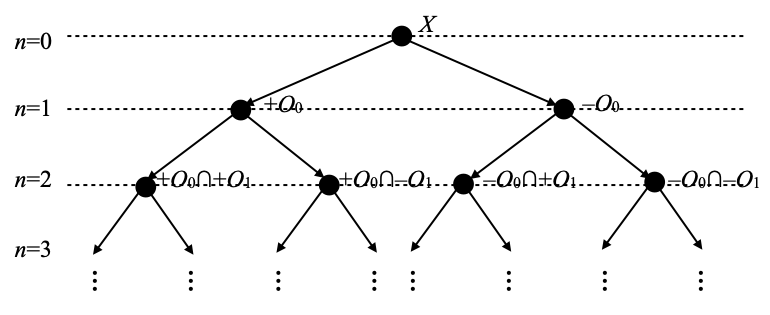
This tree is organized in levels, indexed by natural numbers n, and vertices at level n are labeled with intersections of sets ±O0, ±O1, …, ±On–1, where the signs ± may be chosen independently as + or –. By convention, I will write +Oi for Oi, and –Oi for its complement.
Formally, the vertices of this tree are finite words w over the alphabet ∑≝{+, –}. The level of w is simply its length, and if w is the word ±0 ±1 … ±n–1 where each letter ±i is taken from {+, –}, then we label the vertex w with the clopen set ±0O0 ∩ ±1O1 ∩ … ∩ ±n–1On–1. For example, look at the picture above and consider the word +–. This one sits at level n=2, and is labeled by the clopen set +O0 ∩ –O1.
There are 2n vertices in this tree at level n. In other words, the set ∑n of words of length n over the alphabet ∑ has cardinality 2n. Those vertices are labeled with pairwise disjoint clopen sets, but beware that some may be empty. Deep down in the details of things to come, this would cause some problems (namely, in Lemma E). Costantini and Watson repair this by a kludge (bottom of p.261 and top of p.262, until the end of the proof of Lemma 2 in [4]). Instead, we build a slightly different labeling of our complete binary tree, where vertices may be labeled with clopen sets of the form ±0Oi0 ∩ ±1Oi1 ∩ … ∩ ±n–1Oin–1, with i0, i1, …, in–1 pairwise distinct (in fact, i0<i1<…<in–1, and the point is that indices may fail to be consecutive). We define the label of each vertex w by induction on the length of w as follows. We label the empty word (the root of the tree) with X, as before. This is non-empty… because we have assumed X to be non-empty. If w is labeled with a non-empty clopen set Ow ≝ ±0Oi0 ∩ ±1Oi1 ∩ … ∩ ±n–1Oin–1, then let in be the smallest natural number (necessarily distinct from i0, i1, …, in–1) such that both Ow ∩ +Oin and Ow ∩ –Oin are non-empty. We label the word w+ (w with an additional letter + at the end) by Ow ∩ +Oin and the word w– by Ow ∩ –Oin. We still have to justify that such a number in exists, and we do this as follows. We have seen that our assumptions imply that X has no isolated point, and is T1 (even T2). Since X has no isolated point, and since Ow is non-empty, it cannot contain just one point. Let therefore x and y be two distinct points in Ow. Since X is T1, x has an open neighborhood U that does not contain y. U must contain a basic open set Ok that contains x. Since Ok contains x and not y, k must be distinct from i0, i1, …, in–1, and we define in as the least such k.
I will reuse the notation Ow over and over to denote the (non-empty!) clopen set that labels w, for every vertex w. Although that is not quite completely correct, I will also consider that Ow is equal to ±0O0 ∩ ±1O1 ∩ … ∩ ±n–1On–1 (not the more complex object ±0Oi0 ∩ ±1Oi1 ∩ … ∩ ±n–1Oin–1) if w is the word ±0 ±1 … ±n–1, in examples.
So far so good.
For each natural number n, we will build certain subsets of ∑n, namely we will pick certain families of vertices all sitting at level n, and we will consider the union of their labels. For example, with n=2, if we decide to pick the vertices +–, ––, and –+, then the union of their labels is the union of +O0 ∩ –O1, –O0 ∩ –O1, and –O0 ∩ +O1. In that particular example, note that this union can be simplified to (+O0 ∩ –O1) ∪ –O0, but we will not make such simplifications.
The specific unions of (labels of) vertices all sitting at the same level n that we will pick are the sets ψ(n,f) that we have mentioned earlier; here n varies over the natural numbers, and f are certain functions that will encode which vertices w we pick from ∑n.
The way the functions f are built is technical. First, those functions f are maps from ∑n to {–1, 0, 1}, and the vertices that we will pick are those w ∈ ∑n such that f(w) equals 1 or –1. One may wonder why we need two values, 1 and –1, to do that. Hopefully this will become clearer below; that is needed in order to be able to specify which functions f we will accept as possible arguments of ψ. For reasons that will once again become clearer later, one may think 1 as meaning “possibly taken”, 0 as “not taken”, and –1 as “definitely taken”.
Here is a way of building those functions f. The construction I am going to give is slightly different from Costantini and Watson’s, but not in any essential way; I have not managed to simplify it much.
Let me call a configuration any pair (n, f) where n is a natural number and f is any (for now) function from ∑n to {–1, 0, 1}. We build a directed graph whose set of vertices consists of configurations. A directed graph is simply a binary relation → between configurations, and we define it as follows:
- (n, f) → (m, g) if and only if m>n, and f and g are related as follows:
- (“move of the first kind”) for every w ∈ ∑n such that f(w)=1, then the words ww’ of length m having w as prefix are mapped to 1 by g, except exactly one of them, which is mapped to 0;
- (“move of the second kind”) for every w ∈ ∑n such f(w)=0, then the words ww’ of length m having w as prefix are mapped to 0 by g, except exactly one of them, which is mapped to –1;
- (“move of the third kind”) for every w ∈ ∑n such that f(w)=–1, then all the words ww’ of length m having w as prefix are mapped to –1 by g.
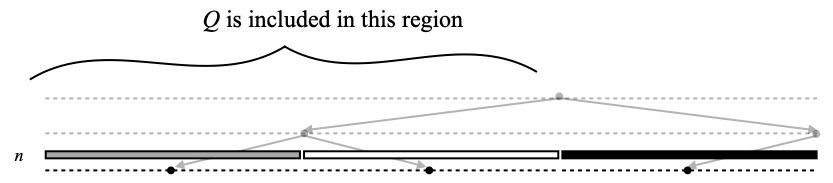
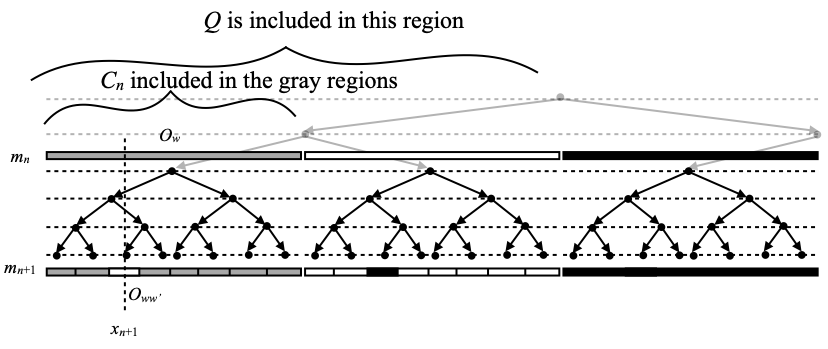
The effect of moves of the first kind (item 1 above) is to make a kind of dent in the clopen set Ow, as selected by f at level n: if w is possibly taken by f (i.e., f(w)=1), then all of its extensions ww’ of length m are still possibly taken by g at level m, except exactly one. Hence g encodes the fact that we chop off one small sliver Oww’ from Ow, and keep the rest as possibly taken. Hopefully the picture below will make this clear. That is the part of the construction needed in order to show that U will contain no subset of the form ■Q, for any compact subset Q of X. (This is where our moves are simpler than Costantini and Watson’s: in their scheme, one would group the clopen chunks on the bottom row in successive pairs, and one would require exactly one chunk of the pair to be possibly taken and the other one to not be taken.)
The effect of moves of the second kind (item 2) is to add back a unique splinter Oww’ as part of the clopen sets that we take wrt. g (and this time, definitely). See the picture below. That is needed in order to show that U is Scott-open.
Finally, moves of the third kind (item 3) are just meant to justify the term ‘definitely taken’, as the following picture should illustrate.
All in all, transitions rewrite all clopen chunks Ow at level n to corresponding unions of smaller clopen chunks at level m, and here is a picture where we have exactly one clopen chunk Ow of each kind:
We define the initial configuration as (0, {ε ↦ 1}). Namely, at level 0, there is a unique vertex, which happens to be the empty word ε, and it is possibly taken. Note that its image by ψ is the whole space X.
Finally, we let Reach denote the set of all configurations (n, f) that are reachable from the initial configuration, namely such that (0, {ε ↦ 1}) →* (n, f), where →* denotes zero, one or more successive → steps. If you prefer, Reach is the smallest set of configurations such that:
- the initial configuration (0, {ε ↦ 1}) is in Reach;
- for every (n, f) in Reach, every configuration (m, g) such that (n, f) → (m, g) is in Reach, too.
We recall that for each configuration (n, f), reachable or not, ψ(n,f) is the union of the sets Ow, where w ranges over the words of ∑n such that f(w) equals 1 or –1 (namely, the union of those sets that are either possibly or definitely taken).
Finally, we define U as the collection of open subsets of X that intersect ψ(n,f) for every reachable configuration (n, f), namely for every (n, f) ∈ Reach.
A useful lemma
For every x ∈ X, and every m ∈ N, let O(x,m) be the unique clopen chunk Ow containing x and such that w has length m. (The set O(x,m) is called V(x,m) in [4], in case you would like to know.) We will keep using the following lemma.
Lemma B. Given any open neighborhood U of x, O(x,m) is included in U for m large enough.
This is due to the fact that the clopen sets Ok form a base of the topology, hence also the sets Ow that label the vertices w. Proving Lemma B formally would involve juggling with all sorts of indices, as in the notation ±0Oi0 ∩ ±1Oi1 ∩ … ∩ ±n–1Oin–1, proving that the way we built those labels ensure that i0<i1<…<in–1, and that for every number k<in–1 distinct from i0, i1, …, in–1, one of the sets ±0Oi0 ∩ ±1Oi1 ∩ … ∩ ±n–1Oin–1 ∩ +Ok and ±0Oi0 ∩ ±1Oi1 ∩ … ∩ ±n–1Oin–1 ∩ –Ok is empty, and the other is equal to ±0Oi0 ∩ ±1Oi1 ∩ … ∩ ±n–1Oin–1, and so on; quite a mess, in my opinion. Hopefully the idea is clear. Costantini and Watson do not make the proof explicit either (see the last paragraph of the proof of Lemma 2 in [4], at the top of page 262.)
Anyway, let us proceed to something more interesting. I guess that the funny definition of the transition relation → was obtained by trial and error, certainly, but that the first productive iteration was in trying to show that U contains no subset of the form ■Q, for any compact subset Q of X, using the argument we explain next.
U contains no subset of the form ■Q, for any compact subset Q of X
In order to show that U contains no subset of the form ■Q, for any compact subset Q of X, we first make a simplifying observation.
Lemma B. U contains ■Q if and only if Q intersects ψ(n,f) for every reachable configuration (n, f).
Proof. This really rests on just the fact that every set ψ(n,f) is closed. If Q intersects ψ(n,f), then every open neighborhood of Q also intersects ψ(n,f), and that proves the if direction. Conversely, if Q does not intersect ψ(n,f), for some reachable configuration (n, f), then it is included in its complement; let us call U that complement, and let us note that U is open (clopen, really). That set U is an open neighborhood of Q that does not intersect ψ(n,f), so ■Q is not included in U. ☐
Now we recall that assumption 2 on X states that every compact subset Q of X is scattered. It is time to recall the game G(Q) of last time:
- C0 ≝ Q; at each round n, player I wins if Cn is empty, otherwise:
- Player I picks an element xn+1 from Cn.
- Player II responds with an open neighborhood Vn+1 of xn+1; let Cn+1 ≝ Cn–Vn+1 and proceed to the next round.
If Q is compact and scattered, then player I has a winning strategy in this game. We will show that if ■Q is included in U, namely if Q intersects ψ(n,f) for every reachable configuration (n, f), then player II has a strategy that prevents player I from winning. This will show that U cannot contain any set ■Q, for any compact (necessarily scattered) subset Q of X.
In the rest of this section, we therefore assume that Q intersects ψ(n,f) for every reachable configuration (n, f).
At the start of the game, we have C0 = Q. Player I immediately wins if that is empty, but it is not. Indeed, since Q intersects ψ(n,f) for every reachable configuration (n, f), it does so in particular for the initial configuration (0, {ε ↦ 1}), whose ψ value is the whole of X. Hence Q intersects X, which means that Q cannot be empty.
Now, we will make sure that player II plays in such a way that the following two invariants are maintained, at each round n:
- (An) Cn is equal to Q ∩ ψ(mn,fn) for some reachable configuration (mn, fn);
- (Bn) Q is disjoint from any set Ow where w has length mn and fn(w)=–1.
(An) implies that Cn will be non-empty (since Q intersects ψ(mn,fn), by assumption), hence that player I cannot win in round n. (Bn) means that whatever clopen chunks Ow were definitely taken in ψ(mn,fn) will be disjoint from Q. As I have said above, the rôle of the chunks that are definitely taken will be to ensure that U is Scott-open. In view of showing that U does not contain ■Q (our current task), those definitely taken chunks are more of a pain in the neck, and invariant (Bn) is there to ensure that they won’t bother us.
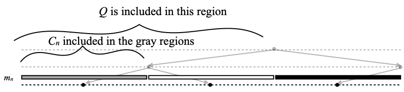
Pictorially, that invariant (Bn) reads as follows:
Additionally, invariant (An) tells us that Cn is equal to Q ∩ ψ(mn,fn), hence that Cn is entirely contained in the gray (possibly taken, mapped by fn to 1) area inside Q.
Initially, namely when n=0, we take (m0, f0) to be the initial configuration (0, {ε ↦ 1}). Then ψ(m0,f0)=X, C0 = Q, so (A0) is true. (B0) is trivial since f0 does not take the value –1.
Now, assume that we are at round n, and that (An) and (Bn) hold. Player I picks an element xn+1 from Cn (hence in one of the possibly taken, gray clopen chunks Ow above), and we now describe how player II will play in order to ensure that Cn+1 = Cn–Vn+1 is equal to Q ∩ ψ(mn+1,fn+1) for some reachable configuration (mn+1, fn+1) satisfying (An+1) and (Bn+1). In order to ensure that (mn+1, fn+1) is reachable, we will simply find it as a successor of (mn, fn); in other words, we will ensure that (mn, fn) → (mn+1, fn+1). As I said earlier, this is probably how this idea of a transition relation → came about.
(An+1) is easy to satisfy. Whatever value of mn+1 > mn we will choose, we can just chop off the small sliver Oww’ around xn+1 from Ow as shown below.
That is a move of the first kind, as used in the definition of the transition relation →. Whatever value for mn+1 we will decide on, we set the unique word w’ of length mn+1–mn such that fn+1(ww’)=0 (this is what chopping off Oww’ really means) by defining it as the unique one such that Oww’=O(xn+1,mn+1).
Let us verify that invariant (An+1) is satisfied. We let player II play the complement of ψ(mn+1,fn+1) for Vn+1, which is open (clopen, really). We have Cn+1 = Cn–Vn+1 by definition of the game, and that is equal to Cn ∩ ψ(mn+1,fn+1) by definition of Vn+1, hence to Cn ∩ ψ(mn,fn) ∩ ψ(mn+1,fn+1) by (An). In order to show that this is equal to Cn ∩ ψ(mn+1,fn+1), it suffices to observe that Cn ∩ ψ(mn+1,fn+1) is included in Cn ∩ ψ(mn,fn) (although ψ(mn+1,fn+1) is not included in ψ(mn+1,fn+1)!). This is because Cn ∩ ψ(mn,fn) is a union of gray chunks at level mn by (An) and (Bn), and all of those are replaced by a union of smaller gray chunks in order to form Cn ∩ ψ(mn+1,fn+1).
(Bn+1) is harder to satisfy, because of the moves of the second kind, namely those by which we replace a clopen chunk that is not taken at level mn (in white) by several smaller clopen chunks at level mn+1, of which exactly one is now definitely taken (in black). See the picture below. (The point zw and the clopen chunk O(zw,mn+1) will be constructed in a moment.)

The trick is to make sure that the new small black chunk added at level level mn+1, is simply disjoint from Q. This is always possible because of Lemma B, once again. Let us see how.
Let Ow be any clopen chunk at level mn that is not taken (formally, w has length mn, and fn(w)=0). Q ∩ Ow is compact, since Ow is closed. If Q ∩ Ow = Ow, then it would be open, since Ow is also open. We recall that X has no non-empty compact open subset: therefore Q ∩ Ow = Ow must be false, since we made sure that Ow is non-empty. This means that Q ∩ Ow is a proper subset of Ow. Hence there is a point zw of Ow that is not in Q. Let us recall that, as a consequence of our assumptions on X, X is T2. Hence the complement U of Q is open. We apply Lemma B, and we find that O(zw,m) is disjoint from Q for m large enough.
Explicitly, there is a natural number kw (let us not forget that it may depend on the given word w of length mn such that fn(w)=0 we started with) such that O(zw,m) is disjoint from Q for every m ≥ kw.
There are only finitely many words w of length mn, so let mn+1 be any natural number larger than or equal to all the numbers kw, where w ranges over the words of length mn such that fn(w)=0 and Ow is non-empty, and also larger than or equal to mn+1. We have obtained that O(zw,mn+1) (contains zw and) is disjoint from Q, for every word w of length mn such that fn(w)=0 and Ow is non-empty, and this secures the part of (Bn+1) that is concerned with moves of the second kind.
In summary, here is how we define (mn+1, fn+1), in such a way that (mn, fn) → (mn+1, fn+1), and (An+1) and (Bn+1) are satisfied. We recall that player I has played a point xn+1 in Cn, that Cn = Q ∩ ψ(mn,fn) by (An), and that Q is disjoint from the black clopen chunks at level mn by (Bn).
- First, we define mn+1 as above, namely larger than or equal to mn+1 and to all the numbers kw, where w ranges over the words of length mn such that fn(w)=0. Then, for every word w of length mn:
- (Moves of the second kind) If fn(w)=0, then we consider the point zw chosen above in Ow–Q. There is a unique word w’ of length mn+1–mn such that Oww’=O(zw,mn+1), the small clopen chunk around zw at level mn+1, and we let fn+1(ww’) ≝ –1 (this chunk is now definitely taken [black], and disjoint from Q, by construction). For all the other words w’ of length mn+1–mn, and as required for moves of the second kind, we let fn+1(ww’) ≝ 0.
- (Moves of the first kind) If the point xn+1 played by player I is in Ow, namely if the word w is the unique word of length mn such that Ow=O(xn+1,mn), then let w’ be the unique word w’ of length mn+1–mn such that Oww’=O(xn+1,mn+1) (the sliver to be chopped off), and we define fn+1(ww’) ≝ 0; otherwise, we pick any word w’ of length mn+1–mn, and let fn+1(ww’) ≝ 0, too. For all the other words w’ of length mn+1–mn, and as required for moves of the first kind, we let fn+1(ww’) ≝ 1 (all the other small clopen chunks remain possibly taken [gray]).
- (Moves of the third kind) There is no choice: we must define fn+1(ww’) as –1 for every word w’ of length mn+1–mn.
The set Vn+1 that player II now plays is the complement of ψ(mn+1,fn+1). We have argued that this was a legal game play, in the sense that Vn+1 is an open neighborhood of xn+1. We have also argued that (An+1) is satisfied. (Bn+1) is satisfied, too, in the sense that Q is still disjoint from the collection of definitely taken clopen chunks with respect to fn+1, simply because those that come from moves of the second kind were chosen disjoint from Q (and those that come from moves of the third kind were already included in chunks that were definitely taken with respect to fn, hence already disjoint from Q by (Bn).) ☐
We are done! Let us sum up. We have assumed that U contained a set of the form ■Q, for some compact set Q. By Lemma B, Q intersects ψ(n,f) for every reachable configuration (n, f). This allowed us to devise a strategy for player II in the game G(Q), by following a sequence of transitions (m0,f0) → (m1,f1) → … → (mn,fn) → …, where (m0,f0) is the initial configuration, and in such a way that, at each round n, Cn is equal to Q ∩ ψ(mn,fn) (by (An)). Since (mn,fn) is reachable, Q intersects ψ(mn,fn), so Cn is not empty, and therefore player I cannot win. However, every compact subset of Q is scattered, so player I has a winning strategy in G(Q). This is a contradiction. This allows us to conclude:
Fact. U contains no set of the form ■Q, for any compact set Q.
U is Scott-open
In order to show that U is Scott-open, we will first require the following two observations about the transition relation →. Those are Lemma 3 and Lemma 4 in [4], respectively, and you can probably see how moves of the second kind were invented in order to ensure that Lemma D would hold.
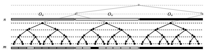
Lemma D. For all configurations (n, g) and (m, f) such that (n, g) → (m, f), for every w ∈ ∑n, Ow intersects ψ(m,f).
Proof. This should be clear from the picture below, where we have shown the three possible cases we have for w; recall that ψ(m,f) is the union of the gray and black regions on the bottom row (level m). Recall that all the clopen chunks involved are non-empty, by construction. ☐
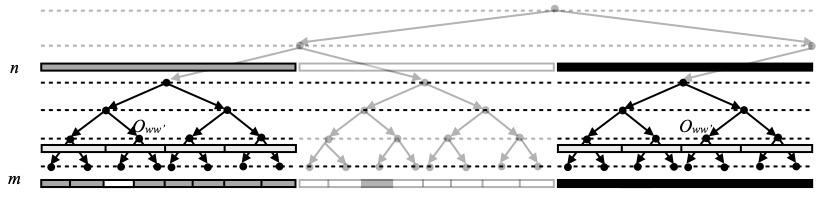
Lemma E. For all configurations (n, g) and (m, f) such that (n, g) → (m, f), for every w ∈ ∑n such that g(w)≠0, for every w’ ∈ ∑m–n–1, Oww’ intersects ψ(m,f).
Proof. This should be obvious from the picture below, where the two possible cases we have for w are when Ow is colored gray (left) or black (right), not white; recall that ψ(m,f) is the union of the gray and black regions on the bottom row (level m). The sets Oww’ that are mentioned in the lemma are those one level above the bottom row, not on the bottom row (those are the small light gray rectangles, and we have shown eight of them). It is important that all those sets Oww’ be non-empty, and this is why we label the vertices of the complete binary tree by non-empty clopen sets only. ☐
Now let us get on to the actual proof. For every net (Ci)i ∈ I, ⊑ of closed subsets of X, we can define its limit superior in the complete lattice of closed subsets of X:
limsupi ∈ I, ⊑ Ci ≝ infi ∈ I supj ⊒ i Cj = ∩i ∈ I cl (∪j ⊒ i Cj)
The closure operator (cl) is needed because suprema in the lattice of closed subsets of X are given by closures of unions. The following will come in handy. I will say that U intersects Ci for cofinally many i ∈ I if and only if for every i ∈ I, there is a j ⊒ i such that U intersects Cj. If I were the set of natural numbers in its usual ordering, that would simply mean that U intersects Ci for infinitely many values of i.
Lemma F. Let (Ci)i ∈ I, ⊑ be a net of closed subsets of X. For every x ∈ X, x is in limsupi ∈ I, ⊑ Ci if and only if every open neighborhood U of x intersects Ci for cofinally many i.
Proof. If x is in limsupi ∈ I, ⊑ Ci, then for every i ∈ I, x is in cl (∪j ⊒ i Cj). Then every open neighborhood of x must intersect cl (∪j ⊒ i Cj), hence also ∪j ⊒ i Cj, hence it must intersect Cj for some j ⊒ i. Conversely, let us assume that every open neighborhood U of x intersects Ci for cofinally many i. In particular, for every open neighborhood U of x, for every i ∈ I, U intersects cl (∪j ⊒ i Cj). If x is not in limsupi ∈ I, ⊑ Ci, then by definition of the limit superior, there is an i ∈ I such that x is not in cl (∪j ⊒ i Cj). Let U be the complement of cl (∪j ⊒ i Cj). That is an open neighborhood of x, and one that does not intersect cl (∪j ⊒ i Cj), and that is impossible. ☐
The reason why limit superiors are important here is because of the following. (In passing, allow me to say that ψ(n,f) is itself a reachable configuration when I mean that this is the value that ψ takes on the reachable configuration (n, f).)
Lemma G. U is Scott-open if and only if for every net (ψ(mi,fi))i ∈ I, ⊑ consisting of reachable configurations, there is a reachable configuration (n, f) such that ψ(n,f) ⊆ limsupi ∈ I, ⊑ ψ(mi,fi).
Proof. Let me recall that U is the collection of all open sets that intersects ψ(n,f) for every reachable configuration (n, f). That is clearly upwards-closed in the inclusion ordering.
Let us first assume that U is Scott-open. For every i ∈ I, let Ui be the complement of cl (∪j ⊒ i ψ(mj,fj)). Then (Ui)i ∈ I, ⊑ is a monotone net of open subsets of X. Moreover, the union U of all the sets Ui is the complement of limsupi ∈ I, ⊑ ψ(mi,fi). We note that no Ui is in U, because Ui does not intersect ψ(mi,fi). Since U is Scott-open, U cannot be in U either. By definition, there must be a reachable configuration (n, f) such that ψ(n,f) does not intersect U. Since U is the complement of limsupi ∈ I, ⊑ ψ(mi,fi), ψ(n,f) must be included in limsupi ∈ I, ⊑ ψ(mi,fi).
In the converse direction, let us assume that U is not Scott-open. There is a monotone net (Ui)i ∈ I, ⊑ of open subsets of X whose union U is in U, and such that no Ui is in U. For every i ∈ I, since Ui is not in U, there is a reachable configuration (mi, fi) such that Ui does not intersect ψ(mi,fi). We claim that there is no reachable configuration (n, f) such that ψ(n,f) ⊆ limsupi ∈ I, ⊑ ψ(mi,fi). Indeed, otherwise, and since U in in U, U would intersect ψ(n,f), say at x. Since U is the union of the sets Ui, at least one of them contains x, call it Uk. By Lemma F, Uk would intersect ψ(mi,fi) for cofinally many i. In particular, Uk would intersect ψ(mi,fi) for some i ⊒ k. But then, Ui, which contains Uk, would also intersect ψ(mi,fi), which is impossible. ☐
In general, given any family A of closed subsets of X, the family {U ∈ OX | U intersects every C ∈ A} is Scott-open if and only if every net (Ci)i ∈ I, ⊑ of elements of A converges to some element C of A in the sense that C ⊆ limsupi ∈ I, ⊑ Ci. This is essentially what we have just proved, in the special case of the family of sets of the form ψ(n,f) with (n, f) reachable. And indeed, limsupi ∈ I, ⊑ Ci is the so-called Kuratowski-Painlevé upper limit of (Ci)i ∈ I, ⊑ in the lattice of closed subsets of X (a notion due to Giuseppe Peano way before Kuratowski and even Painlevé, as it was apparently published in Applicazioni Geometriche, Fratelli Bocca, Torino, 1887; this was regularly mentioned by Szymon Dolecki, see [8]; you can also find an explanation in this document, page 18).
Hence, in order to show that U is Scott-open, we will consider any net (ψ(mi,fi))i ∈ I, ⊑ consisting of reachable configurations, and we will show that there is a reachable configuration (n, f) such that ψ(n,f) ⊆ limsupi ∈ I, ⊑ ψ(mi,fi).
It will be practical to use the following.
- For every subnet (ψ(mα(i’),fα(i’)))i’ ∈ I’, ⪯ of (ψ(mi,fi))i ∈ I, ⊑,
limsupi’ ∈ I’, ⪯ ψ(mα(i’),fα(i’)) ⊆ limsupi ∈ I, ⊑ ψ(mi,fi).
Indeed, by Lemma F, it suffices to observe that every point x in the limit superior on the left, for every open neighborhood U of x, U intersects ψ(mα(i’),fα(i’)) for cofinally many i’, hence U also intersects ψ(mi,fi) for cofinally many i; this is because α is itself cofinal (following Definition 4.7.24 in the book). - In particular, one strategy which we will use repeatedly is to replace (ψ(mi,fi))i ∈ I, ⊑ by a subnet (ψ(mα(i’),fα(i’)))i’ ∈ I’, ⪯. If we manage to find a reachable configuration (n, f) such that ψ(n,f) ⊆ limsupi’ ∈ I’, ⪯ ψ(mα(i’),fα(i’)), then we will immediately obtain that ψ(n,f) ⊆ limsupi ∈ I, ⊑ ψ(mi,fi). We will use that strategy by saying “We pass to the subnet (ψ(mα(i’),fα(i’)))i’ ∈ I’, ⪯“, or simply “by passing to a subnet”, and then we will reason on the subnet, still calling it (ψ(mi,fi))i ∈ I, ⊑.
- As a first application of this strategy, let us imagine that ψ(mi,fi) is ultimately constant, namely that there is an index i0 such that all the sets ψ(mi,fi) with i ⊒ i0 are equal, and let ψ(n,f) be their common value. By passing to the subnet (ψ(mi,fi))i ⊒ i0, ⊑, which is constant and equal to ψ(n,f), hence whose limit superior is equal to ψ(n,f), we obtain that ψ(n,f) ⊆ limsupi ∈ I, ⊑ ψ(mi,fi).
- If there are only finitely many distinct closed sets ψ(mi,fi) when i ranges over I, then one of them occurs cofinally often. In other words, there is at least one set ψ(n,f) such that (n, f)=(mi, fi) for cofinally many i ∈ I. Indeed, otherwise for every set ψ(n,f) among the finitely many that occur in the family (ψ(mi,fi))i ∈ I, there would be an index i(n,f) such that ψ(n,f) cannot occur at any index above i(n,f); since the family of indices is directed, there is an index i above every i(n,f); but then, ψ(mi,fi) cannot occur at any index above i, by construction, which is absurd.
As a second application of our strategy of passing to subnets, we obtain that the result we are after is obvious if there are only finitely many distinct closed sets ψ(mi,fi) when i ranges over I: in that case, one of those sets, ψ(n,f), occurs at positions i that form a cofinal subset I’ of I; we define the sampler α as the inclusion map from I’ into I, and ⪯ as the restriction of ⊑ of I’, then (ψ(mα(i’),fα(i’)))i’ ∈ I’, ⪯ is a subnet of (ψ(mi,fi))i ∈ I, ⊑; but (ψ(mα(i’),fα(i’)))i’ ∈ I’, ⪯ is a constant subnet, since its only element is ψ(n,f), and therefore ψ(n,f) = limsupi’ ∈ I’, ⪯ ψ(mα(i’),fα(i’)). Hence, by passing to that subnet, we obtain that ψ(n,f) ⊆ limsupi ∈ I, ⊑ ψ(mi,fi).
All right, so let us consider any net (ψ(mi,fi))i ∈ I, ⊑ consisting of reachable configurations.
If the levels mi are bounded, namely if there is a constant k such that mi≤k for every i ∈ I, then there are only finitely many values that mi can take. Additionally, for a fixed value mi, there are only finitely many choices for fi : ∑mi → {–1, 0, 1}. Hence there are only finitely many distinct pairs (mi ,fi), and therefore also only finitely many distinct sets ψ(mi,fi). We have just seen that there is a reachable configuration (n, f) such that ψ(n,f) ⊆ limsupi ∈ I, ⊑ ψ(mi,fi) in that case.
So let us concentrate on the more interesting case where there is no upper bound on the levels mi.
If ψ(mi,fi) is the (ψ value of the) initial configuration for i large enough, then (ψ(mi,fi))i ∈ I, ⊑ is, in particular, ultimately constant, and we have seen that the result was true in this case.
Hence we will assume that it is not the case that ψ(mi,fi) is the initial configuration for i large enough, namely that ψ(mi,fi) is distinct from the initial configuration for cofinally many i. (Think about it: “not (for i large enough, P(i))” is equivalent to “for cofinally many i, not P(i)”.) By passing to subnets, we may assume that none of the configurations ψ(mi,fi) is the initial configuration.
This entails that each (mi,fi) is the successor of some other configuration (ni,gi). Namely, (ni,gi) → (mi,fi) for every i ∈ I.
If the numbers ni are not bounded from above, then we claim that limsupi ∈ I, ⊑ ψ(mi,fi) = X. By Lemma F, it suffices to verify that for every x ∈ X, for every open neighborhood U of x, U intersects ψ(mi,fi) for cofinally many i. It is time to recall Lemma B: for every m ∈ N, we have used the notation O(x,n) to denote the unique clopen chunk Ow containing x and such that w has length n, and we have shown that O(x,n) is included in U for n large enough, say n≥k0. The subfamily of those indices i ∈ I such that ni≥k0 is cofinal, since the numbers ni are not bounded from above. Hence, by passing to a subnet, we may assume that O(x,ni) is included in U for every i ∈ I. For each fixed i ∈ I, O(x,ni) is a clopen chunk Ow, and (ni,gi) → (mi,fi), so by Lemma D, O(x,ni) intersects ψ(mi,fi). It follows that the larger set U also intersects ψ(mi,fi). This concludes our argument that limsupi ∈ I, ⊑ ψ(mi,fi) = X. In particular, ψ(n,f) ⊆ limsupi ∈ I, ⊑ ψ(mi,fi) for any reachable configuration (n, f), for example for the initial configuration.
It remains to deal with the case where the numbers ni are bounded from above. Then there are only finitely many configurations (ni, gi), when i ranges over I. Hence, by passing to a subnet, we may assume that they are all equal; the argument is the same as the one we used when we assumed that the numbers mi were bounded from above. Therefore (and this is the last case to be examined!) we may assume that all the configurations (ni, gi) are equal to a unique configuration (n, g). Then (n,g) → (mi,fi) for every i ∈ I. We recall that the numbers mi are not bounded from above.
We will show that ψ(n,g) ⊆ limsupi ∈ I, ⊑ ψ(mi,fi), with the choice of reachable configuration (n,g) that we have just made. Once again we rely on Lemma F: we claim that for every x ∈ ψ(n,g), for every open neighborhood U of x, U intersects ψ(mi,fi) for cofinally many i. We will really show the stronger statement that given any open neighborhood U of x, U intersects ψ(mi,fi) for all indices i provided that they large enough. We start by using Lemma B: for some m≥n large enough, O(x,m) is an open neighborhood of x included in U. Let w be the unique word of length m such that Ow=O(x,m). Since the numbers mi are unbounded, the subfamily of indices i such that mi>m is cofinal. Hence, passing to a subnet, we will assume that mi>n for every i ∈ I. By Lemma E, recalling that (n, g) → (mi, fi), and noticing that g(w)≠0 (since x is in ψ(n,g), namely in some gray or black clopen chunk relative to g), we obtain that for every w’ ∈ ∑mi–n–1, Oww’ intersects ψ(mi,fi), for every i ∈ I. For each i, we pick any such w’ (we can even require Oww’ to contain x, which seems natural, but is not required), and we notice that Oww’ is included in Ow, hence in U. Therefore U intersects ψ(mi,fi), for every i ∈ I.
We have finally obtained:
Fact. U is Scott-open.
This concludes our entire proof, following Costantini and Watson’s argument [4].
Conclusion
Let me sum up what we have proved.
Theorem [4]. Let X be a non-empty topological space that is:
- second-countable, zero-dimensional,
- in which every compact subset is scattered,
- and with no non-empty compact open subset.
Equivalently, let X be a zero-dimensional metrizable space in which every compact subset is scattered, and with no isolated point.
Then there is a Scott-open subset U of OX that contains no subset of the form ■Q, for any compact subset Q of X. In particular, X is not consonant.
As a corollary, Q is not consonant.
One may wonder whether that theorem would apply to other spaces than Q. Well, of course: for example, it applies to the subspace of rational numbers between 0 and 1, but is there any fundamentally different space to which this theorem applies?
For example, this theorem does not apply to the other famously non-consonant space, the Sorgenfrey line Rℓ. That is a zero-dimensional space, in which every compact subset is scattered (given the explicit shape of compact subsets Q of Rℓ, player I wins the game G(Q) by always picking the leftmost point of Q: exercise!), and with no non-empty compact open subset (again, look at the shape of compact subsets). However, Rℓ is not second-countable (and not metrizable). Is there a way of modifying the Costantini-Watson argument in such a way that we could weaken the assumption of second-countability to first-countability, or to first-countability and being hereditarily Lindelöf for example?
- Szymon Dolecki, Gabriele H. Greco, and Alojzy Lechicki, 1995. When do the upper Kuratowski topology (homeomorphically, Scott topology) and the co-compact topology coincide? Transactions of the American Mathematical Society, 347(8), 2869–2884.
- Ahmed Bouziad, Borel measures in consonant spaces, Topology and its Applications 70 (1996), 125—138.
- David Preiss. Spaces in which Prohorov’s theorem is not valid. Zeitschrift für Wahrscheinlichkeitstheorie und Verwandte Gebiete 27 (1973), 109—116.
- Camillo Costantini and Stephen Watson, On the dissonance of some metrizable spaces, Topology and its Applications 84 (1998), 259—268.
- Matthew de Brecht, Jean Goubault-Larrecq, Xiaodong Jia, and Zhenchao Lyu. Domain-complete and LCS-complete Spaces. In Proceedings of the International Symposium on Domain Theory (ISDT’19), volume 345 of Electronic Notes in Theoretical Computer Science, pages 3–35, Yangzhou, China, June 2019. Elsevier Science Publishers. doi:10.1016/j.entcs.2019.07.014.
- Matthew de Brecht and Tatsuji Kawai. On the commutativity of the powerspace constructions. Logical Methods in Computer Science, 15(3), 2019.
- Peter T. Johnstone and Stephen Vickers. Preframe presentations present. In A. Carboni, M.C. Pedicchio and G. Rosolini (eds), Category Theory (Proceedings, Como 1990), Lecture Notes in Mathematics, 1488:193–212, 1991.
- Dolecki, Szymon, Greco, Gabriele H, 2010. Towards Historical Roots of Necessary Conditions of Optimality: Regula of Peano. Dedicated to professor Stefan Rolewicz on his 75-th birthday and Commemorating the 150-th anniversary of the birth of Giuseppe Peano.

— Jean Goubault-Larrecq (June 20th, 2022)