The Sorgenfrey line is not consonant

I have already talked about consonant spaces, for example here. A space X is consonant [1] if and only if the compact-open topology and the Isbell topology coincide on the function space [X → Y] for every topological space Y. It is equivalent to require that they coincide on the single function space [X → S], where S is Sierpiński space {0 < 1}. Since a continuous map from X to S is the characteristic map of a unique open subset of X, X is consonant if and only if every Scott-open subset U of the lattice OX of open subsets of X is a union of sets of the form ■Q≝{U | Q ⊆ U}, where the sets Q are compact saturated subsets of X.

In Exercise 5.4.12 of the book, I ask the reader to prove that neither the space of rationals, Q, nor the Sorgenfrey line, R_ℓ, is consonant. That is what I classified as the important blooper #5 in the list of errata, because the proof I had originally in mind was too simple-minded to have any chance of succeeding. But showing that R_ℓ is not consonant is not that hard, finally. I will explain the argument. This will also be an excuse to explain some additional topological properties of R_ℓ.

The fact that R_ℓ is not consonant was proved by Costantini and Watson, as a consequence of a more general result [3]. (Update, April 22nd, 2022: no, Costantini and Watson’s theorem does not apply. Instead, the fact that R_ℓ is not consonant is due to Alleche and Calbrix [8]. Sorry for the confusion.) Instead, the route I will take has some similarities with what Bouziad did in [2] in order to prove that Q is not consonant—again, as consequence of a more general result—in the sense that I will rely on a bit of measure theory. (Update, April 22nd, 2022. And indeed, the argument I will develop below is essentially Alleche and Calbrix’s.) If you don’t know anything about measure theory, I will also give an argument that only requires some domain theory, most of which is in appendices, at the end of this post.

The Sorgenfrey line R_ℓ

Before we start, let me recall what the Sorgenfrey line R_ℓ is.

It is an incredible beast. Its points are just the real numbers, but its topology is generated by the half-open intervals [a,b[ with a < b. The topology of R_ℓ is finer than the usual metric topology of R. R_ℓ is a zero- dimensional, first-countable space (Exercices 4.1.34, 4.7.17 in the book). It is paracompact hence T₄, and Choquet-complete hence a Baire space (Exercises 6.3.32, 7.6.11). R_ℓ is not locally compact, as every compact subset of R_ℓ has empty interior (Exercise 4.8.5). Although it is first-countable, R_ℓ is not second-countable (Exercise 6.3.10).

We won’t need any of that! It is enough to remember that R_ℓ exhibits a mixture of the nice (paracompact, T₄, Choquet-complete, Baire, first-countable) and of the ugly (not locally compact, not second-countable). We will add some new water to the pot of ugliness (non consonant), and also to the jar of niceness (hereditary Lindelöf, see below).

R_ℓ is not consonant: the short argument

We consider the collection U of open subsets of R_ℓ whose Lebesgue measure is > r, for some fixed r>0. That is a Scott-open subset of O(R_ℓ), and a non-empty one, too (since [–r, r[ is in U, for example), but we claim that it simply contains no subset of the form ■Q for any compact (saturated) subset of R_ℓ. Hence U is certainly not a union of sets of the form ■Q.

In order to see this, we realize that every compact subset Q of R_ℓ is countable. Writing Q as {x₀, x₁, …, x_n, …}, we see that U ≝ ∪_{n ∈ N} [x_n, ε/2ⁿ[ is an open neighborhood of Q for every ε>0, namely that U in in ■Q. However the Lebesgue measure of U is smaller than or equal to ∑_{n ∈ N} ε/2ⁿ = 2ε, so U cannot be in U as soon as we pick ε≤r/2.

Now, wait! I skipped a number of details here. One is that I have not said why every compact subset Q of R_ℓ is countable. This is what I am going to show next, and, while we are at it, I will give a complete characterization of the compact subsets of R_ℓ. Another missing piece is the reason why U is Scott-open. That would be the case is the Lebesgue measure of any directed union of open sets were equal to the supremum of their measures, but measures only satisfy this property for countable directed unions in general. The measures that satisfy this property for arbitrary unions are called τ-smooth. Here a miracle will occur, thanks to a theorem due to Wolfgang Adamski [4], and a magical property called hereditary Lindelöfness, which I will talk about, too. This all uses a bit of measure theory, but, if you have never heard about measure theory, I will give you a purely domain-theoretic construction of U in Appendix B at the end of this post.

The compact subsets of the Sorgenfrey line are countable

Every compact subset Q of R_ℓ is countable, and this is easy to see.

nWe first note that the sets ]−∞,r–ε[ and [r, +∞[ are open, for all r and ε, because they are unions of basic open sets [r–ε–n–1, r–ε–n[, n ∈ N, and of [r+n, r+n+1[, n ∈ N, respectively.

Next, given a compact subset Q of R_ℓ, we realize that, for every r in Q, the open sets ]−∞,r–ε[ with ε>0, plus [r, +∞[, form an open cover of Q. (Indeed, of the whole of R_ℓ!) We extract a finite subcover: without loss of generality, we may assume that this subcover contains [r, +∞[, otherwise we add it back; the other elements of the subcover are ]−∞,r–ε₁[, …, ]−∞,r–ε_n[. We ick ε>0 so that ε<ε₁, …, ε_n, and we see that Q is included in ]−∞,r–ε[ ∪ [r, +∞[, namely that it does not intersect [r–ε, r[. In order to display the dependency on r, let us write ε_r for that ε.

Let us pick a rational number q_r in [r–ε_r, r[, one for each r in Q. The map r ∈ Q ↦ q_r is injective: otherwise there would be two distinct elements r and s of Q such that [r–ε_r, r[ and [s–ε_s, s[ would overlap (at q_r=q_s). By symmetry, let us assume r<s. Then r would be in [s–ε_s, s[, which is impossible since r is in Q but [s–ε_s, s[ does not intersect Q.

We have built an injective map from Q to the set of rationals, which is countable. Therefore Q is countable.

That much is enough knowledge for us on the compact subsets of R_ℓ. However, it would be foolish to stop here and not investigate the nature of compact subsets of R_ℓ, right? Hence, let us embark on characterizing the compact subsets of R_ℓ exactly.

Characterizing the compact subsets of the Sorgenfrey line

Here is another property of compact subsets of R_ℓ that can be proved in a similar way as above.

Fact A. Every compact subset Q of R_ℓ is well-founded with respect to ≥: there is no infinite chain of the form r₀ < r₁ < … < r_n < … in Q.

Proof. Let r ≝ sup_n∈N r_n. Then the open sets ]−∞,r₀[, [r₀,r₁[, …, [r_n,r_n+1[, …, together with [r,+∞[ in case that r≠+∞, would form an open cover of Q without a finite subcover. ☐

Fact A says that every compact subset of R_ℓ is a well-founded subset of (R, ≥), namely of R with the opposite ≥ of the usual ordering ≤.

A directed family in (R, ≥) is a filtered family: a non-empty family in which for any two elements, there is an element less than or equal to both; and “filtered” in not even necessary, since the ordering ≤ on R is total: in other words, a filtered family is just a non-empty family there.

Fact B. Every compact subset Q of R_ℓ is a subdcpo of (R, ≥): the infimum, taken in R, of every filtered family of elements of Q lies in Q.

Proof. We first need to note that a net (x_i)_i∈I,⊑ converges to x in R_ℓ if and only if x_i tends to x from the right, namely: for every ε > 0, x ≤ x_i < x + ε for i large enough. This is Exercise 4.7.6 in the book, but the argument is very short, and I will let you verify this by yourselves.

Let D be any non-empty subset of Q, and let r ≝ inf D. Since the topology of R_ℓ is finer than the topology of R, every compact subset of R_ℓ is also compact in R, in particular, it is bounded. Therefore r is a well-defined real number (not –∞).

By Fact A, Q is well-founded, so D is isomorphic to a unique ordinal β, and we can write the elements of D as r_α, α<β, in such a way that for all α,α′ <β, α≤α′ if and only if r_α ≥ r_α’. The net (r_α)_α<β,≤ then converges to r from the right. Since R_ℓ is T₂, its compact subset Q is closed, so r is in Q. ☐

Note that, if the compact set Q is non-empty, then in particular inf Q lies in Q, namely, Q has a least element. That could also be derived from the fact that every compact subset of R_ℓ is compact in R.

Here is an example of a compact subset of R_ℓ: the set of points of the form 1/2ⁿ, n ∈ N, plus the point zero. We can index those points by ordinal numbers: point number n is 1/2ⁿ, and there is an additional point numbered ω, which is zero:

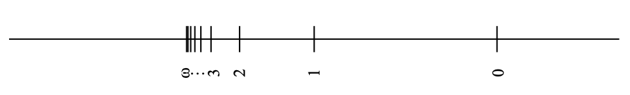
Every well-founded subset of (R, ≥) must be isomorphic to an ordinal (here, ω+1: an ordinal is also the set of all the ordinals strictly below it, so ω+1 = {0, 1, …, n, …, ω}.) Hence if Q is a compact subset of R_ℓ, then its elements must be numbered by ordinal numbers, from right to left, as in the above picture. Additionally, since Q is a subdcpo, that enumeration must stop at some ordinal (Q has a least element), and points of Q must cluster towards points which are numbered with a limit ordinal (from the right), as in the above picture where points cluster towards point number ω, coming from the right.

There are more complex compact subsets, such as the following one, whose points are indexed by the ordinals from 0 to ω².

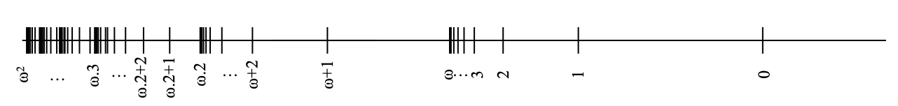
How do I know that the latter is compact in R_ℓ? Well, here is a complete characterization.

Proposition C. The compact subsets of the Sorgenfrey line R_ℓ are exactly the well-founded subdcpos of (R, ≥).

Proof. Considering Facts A and B, it suffices to show that every well-founded subdcpo Q of (R, ≥) is compact in R_ℓ. We use Alexander’s subbase lemma (Theorem 4.4.29 in the book): for every family U of basic open subsets that covers Q, we will extract a finite subcover. We build a (finite or infinite) sequence of elements r_n of Q and another sequence of elements [a_n,b_n[ of U by induction on n in such a way that:

1. r₀ < r₁ < … < r_n < … (so yes, the sequence will in fact be finite, since Q is well-founded in (R, ≥), but let us not go too fast);
2. for each n, r_n is in [a_n,b_n[;
3. for each n, the intervals [a₀,b₀[, …, [a_n,b_n[ cover all the elements of Q that are ≤r_n; in other words, every element of Q is in [a₀,b₀[ ∪ … ∪ [a_n,b_n[ ∪ ]r_n,+∞[.

In the base case (n=0), we take r₀≝inf Q, which is in Q since Q is a subdcpo of (R, ≥). Being in Q, r₀ is in some basic open subset [a₀,b₀[ ∈ U. We then note that every element of Q is in [a₀,b₀[ ∪ ]r₀,+∞[.

In the induction case (n≥1), we assume we already have elements r₀ < r₁ < … < r_n–1 in Q, lying in [a₀,b₀[, …, [a_n–1,b_n–1[ respectively, and such that every element of Q is in [a₀,b₀[ ∪ … ∪ [a_n–1,b_n–1[ or is >r_n–1. Let Q_n be Q – ([a₀,b₀[ ∪ … ∪ [a_n–1,b_n–1[). If Q_n is empty, then the sequence stops here, namely at r_n–1. Otherwise, Q_n is non-empty hence directed in (R, ≥). Since Q is a subdcpo, inf Q_n exists and is an element of Q. We let r_n≝inf Q_n. Every element of Q_n is >r_n–1, so r_n≥r_n–1. If r_n=r_n–1, then r_n would be in [a_n–1,b_n–1[, in particular a_n–1≤r_n=inf Q_n<b_n–1, so some element of Q_n would be in [a_n–1,b_n–1[, which is impossible. Hence r_n–1<r_n. As far as item 2 is concerned, we merely use the fact that U is a cover of Q, so r_n must be in some [a_n,b_n[ ∈ U. Finally, every element x of Q is in [a₀,b₀[ ∪ … ∪ [a_n–1,b_n–1[ or is >r_n–1. If x>r_n–1, then x is in Q_n, hence x≥r_n, and therefore x is in [a_n,b_n[ or is strictly larger than r_n.

We have built a chain r₀ < r₁ < … < r_n < … of elements of Q satisfying properties 1, 2, and 3 above. Since Q is well-founded, this chain must be finite: the inductive process described above stops at some rank n. In that case Q_n is empty, and therefore Q is included in [a₀,b₀[ ∪ … ∪ [a_n–1,b_n–1[. ☐

In other words, the compact subsets Q of R_ℓ are exactly the set of points x_α enumerated by all ordinals α<β, in such a way that x₀ > x₁ > … > x_n > … > x_ω > x_ω+1 > … > x_ω.2 > …, and so that this forms a subdcpo in the opposite ordering ≥, namely:

• there is a last (smallest with respect to ≤) point in Q, in other words β is not a limit ordinal (in our previous examples, β was equal to ω+1 and to ω²+1 respectively);
• for every chain of points x_α[i] in Q, i ∈ I, inf_{i ∈ I} x_α[i] is again in Q, so must be of the form x_α for some ordinal α<β, and it is easy to see that α must in fact be equal to sup_{i ∈ I} α[i].

The ordinal types of compact subsets of R_ℓ

We have seen that every compact subset of R_ℓ is countable. More general, every well-founded subset E of (R, ≥) is countable. (And similarly with the more usual ordering ≤, too, of course.) That is easy to prove, and we don’t need E to be a subdcpo. For every x in E, we look at the interval ]–∞, x[. If ]–∞, x[ ∩ E is empty, then we pick a rational number q_x in ]–∞, x[. Otherwise, since E is well-founded with respect to ≥, E contains a largest element y (with respect to ≤) that is inside ]–∞, x[. Then we pick a rational number q_x in ]y, x[. The map x ∈ E ↦ q_x is injective: in fact we have y<x if and only if q_y<q_x. Since there are only countably many rational numbers, E is countable.

In particular, the order-type of any compact subset Q of R_ℓ, namely the unique ordinal that is order-isomorphic to (Q, ≥), is a countable ordinal. It is also a non-limit ordinal, because those are exactly the ordinals that are (sub)dcpos. For example, the limit ordinal ω={0, 1, …, n, …} is not a dcpo. But ω+1={0, 1, …, n, …, ω} is a dcpo.

One might wonder which countable ordinals are the order-types of compact subsets of R_ℓ. The answer is simple: all the non-limit countable ordinals. Since I have already spent too much time on compact subsets, I will refer you to Appendix A of this post for details.

The hereditary Lindelöf property

So, enough with the compact subsets of R_ℓ. I promised we would look at a magical property of Lebesgue measure on R_ℓ, and that this would have to do with a property called hereditary Lindelöfness.

A topological space X is hereditarily Lindelöf (train yourself to pronounce that… what a tongue twister!) if and only if every family of open subsets of X contains a countable subfamily with the same union. If you already know what a Lindelöf space is, you may realize that a space is hereditarily Lindelöf if and only if all its subspaces are Lindelöf.

We will see that every second-countable space is hereditarily Lindelöf, and that R_ℓ is an example of a space that is hereditarily Lindelöf… but not second-countable.

Lemma D. Every second-countable space is hereditarily Lindelöf.

Proof. Let X be a second-countable space, and B be a countable base of its topology. Let (U_i)_{i ∈ I} be an arbitrary family of open subsets of X, and let U be its union. For every point x of U, there is an index i in I such that x is in U_i, let us call it i[x]. Also, there is an element B[x] of the base B such that x ∈ B[x] ⊆ U_i[x]. Then U ⊆ ∪_{x ∈ U} B[x]. However, since B is countable, the latter is a countable union. In other words, for each element of the base B that arises as B[x] for some x in U, we pick such a point x; we collect all those points and form a countable subset E of U; then U ⊆ ∪_{x ∈ E} B[x]. Now ∪_{x ∈ E} B[x] ⊆ ∪_{x ∈ E} U_i[x] ⊆ U, so U = ∪_{x ∈ E} B[x] = ∪_{x ∈ E} U_i[x]: when x ranges over the set E, the open sets U_i[x] form a countable subfamily of (U_i)_{i ∈ I} with the same union, namely U. ☐

The Sorgenfrey line R_ℓ is not second-countable: you can find the argument in Exercise 6.3.10 of the book. Rather amazingly, we have the following.

Proposition E. R_ℓ is hereditarily Lindelöf.

Proof. I took the proof from the Math Stack exchange. Let us agree to write Ů for the interior of a set U in the topology of R: not that of R_ℓ, please bear that in mind.

Let (U_i)_{i ∈ I} be any family of open subsets of R_ℓ, let U be its union and let U’ denote the union ∪_{i ∈ I} Ů_i of their interiors in the topology of R. Since R is second-countable, hence hereditarily Lindelöf by Lemma D, there is a countable subset J of I such that U’ = ∪_{i ∈ J} Ů_i.

We claim that U–U’ is countable. For each point x ∈ U–U’, x is in some U_i, hence in some basic open subset [a_x, b_x[ ⊆ U_i. Then x is also included in the smaller basic open set [x, b_x[. The (fully) open interval ]x, b_x[ is included in Ů_i, hence in U’. By picking a rational number q_x in [x, b_x[ for each x ∈ U–U’, we see that there are only countably many distinct intervals [x, b_x[. For any two distinct points x and y of U–U’, if the intervals [x, b_x[ and [y, b_y[ overlapped, then either y would be in [x, b_x[ or x would be in [y, b_y[. Let us imagine that y is in [x, b_x[. Since y≠x, y must be in ]x, b_x[ ⊆ U’; that is impossible since we have chosen y in U–U’. We reason similarly if x is in [y, b_y[. We have shown that for any two distinct points x and y of U–U’, the intervals [x, b_x[ and [y, b_y[ do not overlap; in particular, they are distinct. As there are only countably many such intervals, there are only countably many points in U–U’.

For each x ∈ U–U’, let us pick an index i[x] in I such that x is in U_i[x]. Let K be {i[x] | x ∈ U–U’}. This is a countable set, and therefore so is J ∪ K. The countable subfamily consisting of those sets U_i such that i ∈ J ∪ K then covers both U’ and U–U’, hence it covers the whole of U. It follows that U = ∪_{i ∈ J ∪ K} U_i. ☐

Hence R_ℓ once again serves as a counterexample! Namely, as an example that not all hereditarily Lindelöf spaces are second-countable.

Before we proceed, let me mention the following practical fact.

Lemma F. A space X is hereditarily Lindelöf if and only if every directed family (U_i)_{i ∈ I} of open sets contains an ascending subsequence U_i[0] ⊆ U_i[1] ⊆ … ⊆ U_i[n] ⊆ … with the same union.

Proof. If X is hereditary Lindelöf, then we can assume that I is countable, and even that I is just N. We build i[n] by induction on n as follows. We let i[0]≝0. For every n≥1, we define i[n] as any index i such that U_i contains U_i[n–1] and U_n. It is easy to see that U_i[0] ⊆ U_i[1] ⊆ … ⊆ U_i[n] ⊆ … Moreover, for every natural number n, U_n is included in U_i[n], so that the union of the sets U_i[n] contains the union of the sets U_n, and is therefore equal to it.

Conversely, let us assume that every directed family of open sets contains an ascending subsequence with the same union. Let (U_i)_{i ∈ I} be any family of open sets, and U be its union. For every non-empty finite subset J of I, let U_J ≝ ∪_{i ∈ J} U_i: the family (U_J)_{J finite non-empty ⊆ I} is now directed, its union is U, and by assumption we can find an ascending subsequence U_J[0] ⊆ U_J[1] ⊆ … ⊆ U_J[n] ⊆ … whose union is U. It follows that the union of the sets U_i, where i ranges over the countable family ∪_{n ∈ N} J[n], is equal to U. ☐

The Lebesgue measure on R_ℓ

If you know about Lebesgue measure λ, proving that R_ℓ is not consonant is now only a few steps away. (If you don’t, then stop reading here and proceed directly to Appendix B.) Realizing that every open subset of R_ℓ is a countable union of basic open subsets [a,b[ (a simple consequence of the fact that R_ℓ is hereditarily Lindelöf), and that any subset of the form [a,b[ is a Borel subset of R, we see that R and R_ℓ have the same Borel σ-algebras. In particular, λ defines a Borel measure on R_ℓ.

Then we notice that every Borel measure on a hereditarily Lindelöf space is τ-smooth [4]. This is much easier to understand and prove than the intimidating wording would leave us to believe. A measure is τ-smooth if and only if its restriction to the lattice of open sets is Scott-continuous. If X is a hereditarily Lindelöf space, then for every directed family (U_i)_{i ∈ I} of open subsets of X, with union U, there is an ascending subsequence U_i[0] ⊆ U_i[1] ⊆ … ⊆ U_i[n] ⊆ … whose union is also U (see Lemma F). Given any Borel measure μ on X, μ(U) is then equal to μ(∪_{n ∈ N} U_i[n]). Since the union ∪_{n ∈ N} U_i[n] is a union of a countable chain, the fact that μ is a measure entails that μ(U) = sup_{n ∈ N} μ(U_i[n]), and one easily checks that this is also equal to sup_{i ∈ I} μ(U_i). The important point is that measures commute with suprema of countable chains. Going from the countable case to the general case is something we can afford thanks to hereditary Lindelöfness.

By the way, hereditary Lindelöfness is a sufficient and necessary condition: as Adamski proved, a space X is hereditarily Lindelöf if and only if every Borel measure on X is τ-smooth [4].

In any case, Lebesgue measure λ is a Borel measure on R_ℓ. R_ℓ is hereditarily Lindelöf by Proposition E, and Adamski’s theorem tells us that λ is τ-smooth, namely that it restricts to a Scott-continuous map from O(R_ℓ) to R₊ ∪ {+∞}. It follows that the set U of all open subsets U of R_ℓ such that λ(U)>r (for any given r>0) is Scott-open, as promised. That was the only remaining detail we had to fill in the argument we gave at the beginning of this post: R_ℓ is not consonant.

That’s it! Oh, if you’re not completely exhausted, have a look at Appendix B for a funny purely domain-theoretic of building the same Scott-open family U.

1. Szymon Dolecki, Gabriele H. Greco, and Alojzy Lechicki, 1995. When do the upper Kuratowski topology (homeomorphically, Scott topology) and the co-compact topology coincide? Transactions of the American Mathematical Society, 347(8), 2869–2884.
2. Ahmed Bouziad, Borel measures in consonant spaces, Topology and its Applications 70 (1996), 125—138.
3. Camillo Costantini and Stephen Watson, On the dissonance of some metrizable spaces, Topology and its Applications 84 (1998), 259—268.
4. Wolfgang Adamski. τ-smooth Borel measures on topological spaces. Mathematische Nachrichten, 78:97–107, 1977.
5. Claire Jones. Probabilistic Non-Determinism. Ph.D. thesis, University of Edinburgh. Technical Report ECS-LFCS-90-105, 1990.
6. Nait Saheb-Djahromi. Cpo’s of Measures for Nondeterminism. Theoretical Computer Science, 12, pages 19–37, 1980.
7. Jimmie Lawson. Valuations in continuous lattices. In: Hoffman, R.-E. (ed.), Continuous Lattices and Related Topics. Mathematik Arbeitspapiere, Universität Bremen 27, 1982.
8. Boualem Alleche and Jean Calbrix. On the coincidence of the upper Kuratowski topology with the cocompact topology. Topology and its Applications 93(3):207—218, 1999.

Appendix A

We show that every countable non-limit ordinal β+1 is the order-type of some compact subset Q_β of R_ℓ. (Technically, 0 is another non-limit ordinal, and it is not of the form β+1; but 0 if of course the order-type of the empty compact set.) In fact, we will show that we can even design Q_β so that it is included in any prescribed interval ]a,b], a<b.

In order to show this, we need to know the following interesting little fact: every countable limit ordinal has cofinality ω. This is savant jargon to say that every countable limit ordinal β is the supremum of a monotone sequence of ordinals α₀ ≤ α₁ ≤ … ≤ α_n ≤ … < β indexed by natural numbers. Here is how you prove it. First, β is the supremum of all the ordinals α<β. The family of those ordinals is just β itself, and is therefore countable. This gives us an enumeration of the ordinals α<β by natural numbers; but we are not done yet, because that enumeration may fail to be monotone. So we have to work a bit more. Let f be a bijection between N and β. This is the enumeration we have just talked about. We define α_n by induction on n, as being f(m) where m is the first natural number ≥m such that f(m) is strictly larger than all the previously defined ordinals α₀, α₁, …, α_n–1. I’ll let you check by yourselves that the sequence of ordinals α_n is well-defined, monotone, and cofinal in the family of all ordinals α<β, so that its supremum is β as well.

We can now build Q_β (compact in R_ℓ, of order-type β+1, and included in ]a,b], a<b) by induction on β.

• If β=0, then we take Q_β ≝ {b}.
• If β is a successor ordinal, say β=γ+1, then by induction hypothesis we have already formed Q_γ, and we may assume that Q_γ is included in ]a,b]. Then Q_β ≝ Q_γ ∪ {(a+min Q_γ)/2} suits our needs.
• Finally, let us assume that β is a (countable) limit ordinal. First, we express β as the supremum of a monotone sequence of ordinals α₀ ≤ α₁ ≤ … ≤ α_n ≤ … < β, using the fact that every countable limit ordinal has cofinality ω. We let β[0]≝α₀. For every n≥1, the set of ordinals between α_n–1 (included) and α_n (excluded) is well-founded and total, hence is isomorphic to a unique ordinal β[n] (its order-type). Clearly, β[n] is countable and smaller than or equal to α_n, hence strictly smaller than β. We can there apply the induction hypothesis: for each n in N, we find a compact subset Q’_n of R_ℓ or order-type β[n] included in ]c+(b–c)/2ⁿ⁺¹, c+(b–c)/2ⁿ], where c is a fixed number in ]a,b], for example (a+b)/2. Let g_n be the order-isomorphism between β[n] and Q’_n. Then we let Q_β be the (disjoint) union of the sets E’_n, for n ∈ N, plus {c}.
  It is easy to see that the order-type of Q_β is β+1. We can even describe an explicit order-isomorphism between β+1 and Q_β: this maps any ordinal α < β[0]=α₀ to g₀(α) the ordinals α₀+α with α < β[1] to g₁(α), the ordinals α₁+α with α < β[2] to g₂(α), and so on; and finally, it maps β to c.
  It remains to show that Q_β is a subdcpo of (R, ≥). Let D be a non-empty family of elements of Q_β. If c is in D, then inf D=c, so inf D is in Q_β. In the rest of the argument, we therefore assume that c is not in D, so that D is included in the union of the compact sets Q’_n, n ∈ N. Let E be the set of natural numbers n such that D contains an element of Q’_n. E is non-empty. If E is bounded, then let n be its largest element. Then D ∩ Q’_n is cofinal in D (with respect to ≥), so inf D = inf (D ∩ Q’_n), and that lies in Q’_n by Fact B, hence in Q_β. If E is unbounded, then there are points of D in intervals ]c+(b–c)/2ⁿ⁺¹, c+(b–c)/2ⁿ] for n arbitrarily large. Then inf D=c, and c is in Q_β.

Appendix B

A continuous valuation on a topological space X is a Scott-continuous map ν : OX → R₊ ∪ {+∞} such that:

• (strictness) ν(∅)=0
• (modularity) ν(U ∪ V) + ν(U ∩ V) = ν(U) + ν(V) for all open subsets U and V of X.

Notions of valuations as strict and modular maps (without Scott-continuity) can be traced back to at least a 1948 paper by Horn and Tarski. Nait Saheb-Djahromi introduced continuous valuations on dcpos in 1980 [6], and Jimmie Lawson proved a fundamental measure extension theorem for continuous valuations in 1982 [7]. Claire Jones’ 1990 PhD thesis [5] popularized the notion among computer scientists, and was probably the first to lay out the general theory of continuous valuations (on dcpos).

Continuous valuations and measures are very close notions. By definition, given any τ-smooth Borel measure μ on X, its restriction to open sets is a continuous valuation. Conversely, there are large classes of spaces on which every continuous valuation extends to a measure on the Borel σ-algebra (Lawson’s paper [7] being the first result of that kind). But enough with measures! I have promised that this section would be purely domain-theoretic.

The collection VX of all continuous valuations on a space X can be ordered by the so-called stochastic ordering: ν≤ν’ if and only if ν(U)≤ν'(U) for every open subset U of X. This turns VX into a dcpo. In order to show the (modularity) law for a directed supremum of continuous valuations, simply observe that + is Scott-continuous on R₊ ∪ {+∞}.

There are some very simple continuous valuations: the Dirac valuation δ_x at x maps every open neighborhood of x to 1, all all other open sets to 0. The finite linear combinations ∑_i=1ⁿ a_i δ_x[i], where each a_i is in R₊, are all continuous valuations. The continuous valuations of this form are called the simple valuations. The probabilistic intuition is that such a continuous valuation represents a process by which we draw x[i] at random with probability a_i (provided the points x[i] are pairwise distinct and the sum of the coefficients a_i equals 1).

Since VX is a dcpo, any directed supremum of simple valuations is a continuous valuation, and I will call the continuous valuations obtained this way quasi-simple. Jones showed that every continuous valuation on a a continuous dcpo is quasi-simple. I am only mentioning this because that is interesting, but we won’t make any use of that here.

We will build a continuous valuation λ on R_ℓ, which is in fact the restriction of Lebesgue measure to the open subsets of R_ℓ. No, λ is not quasi-simple (pardon me for omitting the argument), but the following roundabout strategy will work. We will first embed R_ℓ into a dcpo model, namely a dcpo IR_ℓ in which R_ℓ embeds as the space of its maximal elements. We will then build a certain quasi-simple valuation λ on IR_ℓ, and we will show that λ is supported on its set of maximal elements R_ℓ (in a sense that I will make precise below). It will follow that λ arises in a certain way from a continuous valuation on R_ℓ, and this will be λ.

A dcpo model for R_ℓ

Let IR_ℓ be the following poset. It contains two kinds of points:

• The real numbers r, which will form the set of maximal points of R_ℓ,
• and the half-open intervals [a,b[, with a<b.

We order them as follows:

• [a,b[ ⊑ [a‘,b‘[ if and only if a=a’ and b>b’, namely if and only if [a,b[ contains [a‘,b‘[, and has the same left endpoint;
• [a,b[ ⊑ r for every r ∈ [a,b[;
• the only element larger than or equal to a real number r is r itself.

If you start from an interval [a,b[, the only way to go up from there is to produce intervals [a,b’[ with smaller and smaller values of b’, leaving a untouched, or to directly go from one such interval [a,b’[ to a real number r in [a,b’[ and stop. For example, look at the picture below. If you start from [a,a+1[, you can either go up, geometrically, following the red arrows, or you can go directly to the top line, following the blue arrows, and landing anywhere between a (included) and a+1 (excluded).

It is then easy to see that IR_ℓ is a dcpo. Given any directed family D,

• If D contains some real number r already, then r = sup D;
• Otherwise, D is a family of intervals [a,b_i[, i ∈ I, with the same left end a, and its supremum is the interval [a, inf_{i ∈ I} b_i[ if a<inf_{i ∈ I} b_i, and the real number a otherwise.

The way-below relation on IR_ℓ is given by: A ≪B if and only if B is a real number a, and A is an interval [a, b[ (with the same a). In particular, no interval A is way-below any interval [a, b[: to see this, pick any point r in [a,b[ other than a, then r is the supremum of the chain of intervals [r, r+1/2ⁿ[, n ∈ N, but none of those intervals can be above A. The same argument shows that [a, b[ cannot be way-below any number r in [a,b[ that is different from a. But [a, b[ is way-below a, as one checks easily.

It follows that IR_ℓ is very far from being a continuous dcpo: no interval B can be obtained as the supremum of any directed family (or any family whatsoever) of intervals way-below B.

Still, we have the following. We equip IR_ℓ with the Scott topology of ⊑.

Lemma D. IR_ℓ is a dcpo model of R_ℓ: R_ℓ embeds topologically as the subspace of maximal elements of IR_ℓ.

Proof. Let U be any Scott-open subset of IR_ℓ. We show that U ∩ R_ℓ is open in R_ℓ. In order to see this, let r be any point of U ∩ R_ℓ. Then r is the supremum of the chain [r, r+ε[, ε>0, and is in U, so [r, r+ε[ is an element of U for some ε>0. Since U is upwards-closed, every real number in [r, r+ε[ is in U, hence in U ∩ R_ℓ. This shows that U ∩ R_ℓ is an open neighborhood of r, and since r is arbitrary, U ∩ R_ℓ is open in R_ℓ.

Conversely, we claim that every open subset U of R_ℓ is also open in the subspace topology induced by the inclusion of R_ℓ into IR_ℓ. To this end, it suffices to consider the special case where U is a subbasic open set [a,b[. We consider the set U consisting of all the real numbers in [a,b[, plus all the intervals [a’,b’[ such that a≤a’<b’<b. It is easy to see that U is Scott-open, and that U ∩ R_ℓ=U. ☐

Building λ

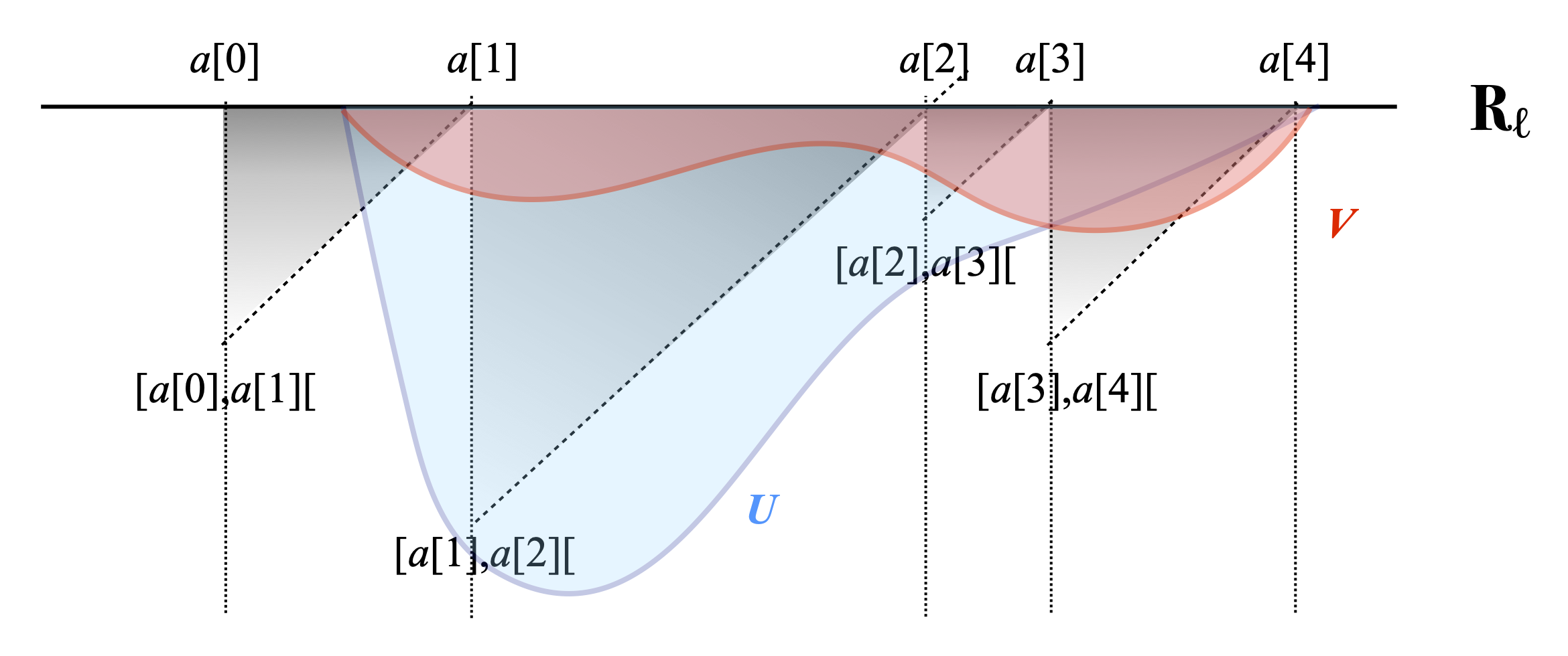
Let us call finite partition (of R_ℓ) any finite list P ≝ {a[0] < a[1] < … < a[n]} of real numbers, n≥1. We view this as a specification of the finitely many pairwise disjoint intervals [a[0], a[1][, …, [a[n–1], a[n][. The lengths of those intervals are (a[1]–a[0]), …, and (a[n]–a[n–1]). With such a finite partition, we associate the simple valuation λ_P ≝ ∑_i=1ⁿ (a[i]–a[i–1]) δ_{[a[i–1], a[i][} on IR_ℓ. Explicitly, for every Scott-open subset U of IR_ℓ, λ_P(U) is the sum of the lengths (a_i–a_i–1) of those intervals [a_i–1, a_i[ which, seen as elements of IR_ℓ, belong to U.

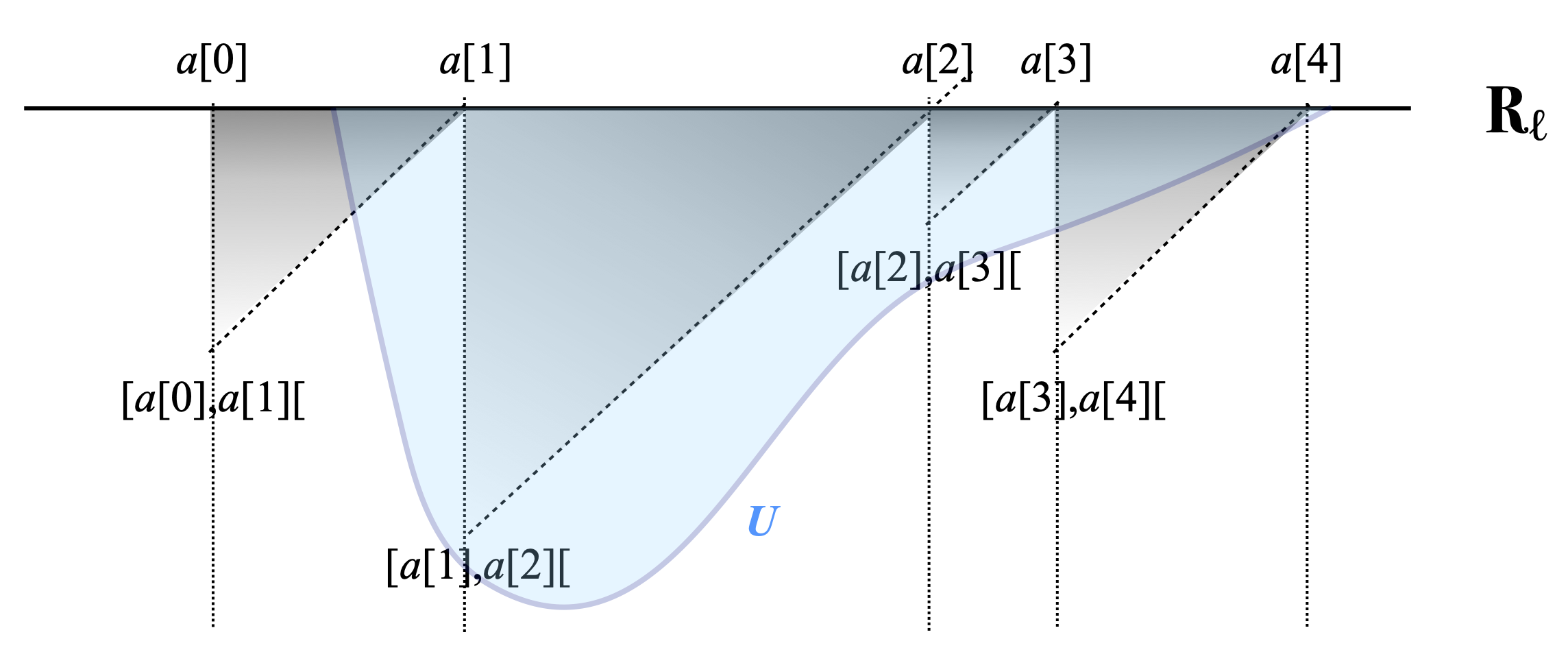
For example, the picture below displays a finite partition P ≝{a[0] < a[1] < a[2] < a[3] < a[4]}, and the corresponding intervals [a[0], a[1][, [a[1], a[2][, [a[2], a[3][, and [a[3], a[4][. Those intervals can be read as strips off the top line, R_ℓ, or as points of IR_ℓ, shown as the (upside-down) tips at the bottom of the corresponding triangles. The picture also displays a Scott-open subset U of IR_ℓ, in a light blue shade. [a[1], a[2][ and [a[2], a[3][ are elements of U, but not [a[0], a[1][ or [a[3], a[4][, and therefore λ_P(U) = a[3]–a[1].

The collection of all finite partitions is directed in the subset ordering ⊆: notably, given any two finite partitions, their union is a finite partition, too.

I claim that the map P ↦ λ_P is monotonic. Let P and Q be two finite partitions, and let us assume that P ⊆ Q. Hence we can write P as {a[0] < a[1] < … < a[n]}, and for each i with 1≤i≤n, we can write the points of Q that lie between a[i–1] and a[i] as b[i,0]≝a[i–1] < b[i,1] < … < b[i,m_i]≝a[i]. For each j with 1≤j≤m_i, the interval [b[i,j–1], b[i,j][ is an element of IR_ℓ that lies above [a[i–1], a[i][, and the sum of the lengths of those intervals [b[i,j–1], b[i,j][, 1≤j≤m_i, is exactly the length (a[i]–a[i–1]) of [a[i–1], a[i][. For every Scott-open subset U of IR_ℓ, λ_P(U) is the sum of the lengths of those intervals [a[i–1], a[i][ that lie in U. Hence λ_P(U) is also the sum of the lengths of the intervals [b[i,j–1], b[i,j][ such that [a[i–1], a[i][ is in U and 1≤j≤m_i. All those intervals [b[i,j–1], b[i,j][ are in U as well, so λ_P(U) is less than or equal to the sum of the lengths of all the intervals [b[i,j–1], b[i,j][ that are in U, when both i and j vary. The latter sum is just λ_Q(U), so λ_P(U)≤λ_Q(U).

Since V(IR_ℓ) is a dcpo, the family of all maps λ_P has a supremum λ.

λ is supported on the set of maximal elements of IR_ℓ

I claim that λ is supported on the set R_ℓ of maximal elements of IR_ℓ. Intuitively, that means that drawing an element at random with respect to λ will give you an element of R_ℓ with probability 1. Formally, that really means that for every fixed open subset U of R_ℓ, and whichever Scott-open subset U of IR_ℓ we consider whose intersection with R_ℓ equals U, λ(U) will always give you the same value, and that will be the desired value λ(U) of the Lebesgue valuation λ on U.

The key to this is Proposition 5.2.28 in the book, a consequence of Rudin’s Lemma. Let me restate it. Given any dcpo X, let Q_fin(X) be the poset of all non-empty finite subsets of X, preordered by the Smyth preordering ≤^#: E ≤^# F if and only if every element of F is above some element of E, namely if and only if ↑E ⊇ ↑F. Proposition 5.2.8 says that, given any directed family (E_i)_{i ∈ I} in Q_fin(X) and any Scott-open subset U of X, if ∩_{i ∈ I} ↑E_i is included in U, then some E_i is included in U already.

Let us say that the endpoints of a finite partition P ≝ {a[0] < a[1] < … < a[n]} are a[0] and a[n]. Let us also write Part(a,b) for the set of all finite partitions whose endpoints are a and b.

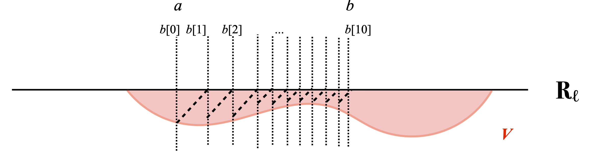
Given any finite partition P ≝ {a[0] < a[1] < … < a[n]}, let us write E_P for the set of intervals [a[0], a[1][, …, [a[n–1], a[n][, viewed as elements of the dcpo IR_ℓ. We observe that, given two finite partitions P and Q in Part (a,b) (hence with the same endpoints a and b), if P ⊆ Q, then E_P ≤^# E_Q. Part (a,b) is a directed family of finite partitions, since {a, b} is in Part (a,b) and Part (a,b) is closed under binary unions. Hence the collection of elements E_P of Q_fin(IR_ℓ) when P varies over Part (a,b) is directed. The intersection of the sets ↑E_P, P ∈ Part (a,b), is exactly the interval [a,b[. By Proposition 5.2.28, we obtain: (*) for every Scott-open subset V of IR_ℓ such that [a,b[ ⊆ V, there is finite partition Q with endpoints a and b such that E_Q is included in V.

This is pictured below. The partition Q is {b[0] < b[1] < … < b[10]}.

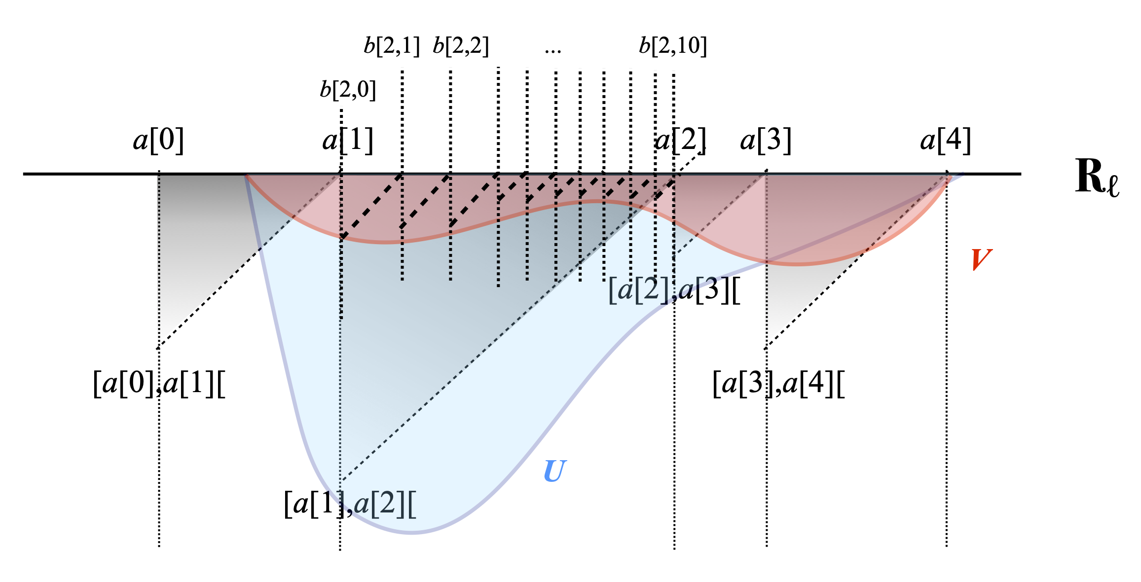
Let U be any open subset of R_ℓ, and let U and V be two Scott-open subsets of IR_ℓ such that U ∩ R_ℓ = V ∩ R_ℓ = U. We wish to show that λ(U)=λ(V). By symmetry, it is enough to show that λ(U)≤λ(V). The situation is exemplified below. Note that U need not be included in V.

In order to show that λ(U)≤λ(V), let r be any positive real number such that r < λ(U). There is a finite partition P such that r < λ_P(U). (You may imagine that this is the partition {a[0] < a[1] < … < a[4]} showed in the picture above.)

We will show that there is a finite partition Q such that r < λ_Q(V). We write P as {a[0] < a[1] < … < a[n]}, and we consider any index i with 1≤i≤n such that [a[i–1], a[i][ is an element of U. (For instance, [a[1], a[2][ in the example above.) Every real number in [a[i–1], a[i][ is above the element [a[i–1], a[i][, hence is also in U. Hence the interval [a[i–1], a[i][ is included in U ∩ R_ℓ, namely in U, and therefore [a[i–1], a[i][ is included in V ∩ R_ℓ, hence in V. By (*), proved above, there is a finite partition Q_i with endpoints a[i–1] and a[i], say Q_i ≝ {b[i,0] < … < b[i,m_i]} (with b[i,0]=a[i–1] and b[i,m_i]=a[i]) such that the intervals [b[i,j–1], b[i,j][, 1≤j≤m_i, are all in V. In the following picture, we show how [a[1], a[2][ is refined by Q₂ ≝ {b[2,0] < … < b[2,10]}.

Let Q be the union of the finite partitions Q_i, when i ranges over the indices i with 1≤i≤n such that [a[i–1], a[i][ is an element of U. If we agree to write those indices i as i[0] < i[1] < … i[n], then the elements of Q are b[i[0],0] < … < b[i[0],m_i[0]] ≤ b[i[1],0] < … < b[i[1],m_i[1]] ≤ … ≤ b[i[n],0] < … < b[i[n],m_i[n]], and E_Q consists of the intervals [b[i,j–1], b[i,j][ with 1≤j≤m_i, and where i can be equal to i[0], i[1], …, or i[n], plus possibly other intervals [b[i[0],m_i[0]], b[i[1],0][, b[i[1],m_i[0]] ≤ b[i[2],0], inbetween two consecutive partitions Q_i. All the intervals of the former kind are in V, from which we conclude that λ_Q(V) is larger than or equal to the sum of their lengths b[i,j]–b[i,j–1]. For each i among i[0], i[1], …, i[n], the sum of the lengths b[i,j]–b[i,j–1], 1≤j≤m_i, is equal to b[i,m_i]–b[i,0] = a[i]–a[i–1], and summing those quantities over i=i[0], i[1], …, i[n] yields λ_P(U). Therefore λ_Q(V)≥λ_P(U)>r.

Defining the Lebesgue valuation λ on R_ℓ

We can therefore define λ(U), for every open subset U of R_ℓ, as λ(U) where U is any Scott-open subset of IR_ℓ such that U ∩ R_ℓ = U.

I claim that λ is a continuous valuation. For every open subset U of R_ℓ, there is at least one Scott-open subset U of IR_ℓ such that U ∩ R_ℓ = U; let me call such a Scott-open set U a representative of U.

• (strictness) the empty subset of IR_ℓ is a representative of the empty subset of R_ℓ, so λ(∅)=λ(∅)=0.
• (modularity) Let U and V be any two open subsets of R_ℓ, with respective representatives U and V. Then U ∪ V is a representative of U ∪ V and U ∩ V is a representative of U ∩ V, so λ(U ∪ V)+λ(U ∩ V)=λ(U ∪ V)+λ(U ∩ V)=λ(U)+λ(V)=λ(U)+λ(V), using the fact that λ is modular in order to justify the middle equation.
• Scott-continuity. We first show that λ is monotonic. Let U and V be any two open subsets of R_ℓ, with respective representatives U and V, and let us assume that U is included in V. It may not be the case that U is included in V, but that does not matter. What does matter is that U ∪ V is another representative of V: (U ∪ V) ∩ R_ℓ = (U ∩ R_ℓ) ∪ (V ∩ R_ℓ) = U ∪ V = V. Therefore λ(V)=λ(U ∪ V)≥λ(U)=λ(U), where the middle inequality is by monotonicity of λ.
  Let us consider any directed family (U_i)_{i ∈ I} of open subsets of R_ℓ, and let their union be U. We consider that directed family as a monotone net, by defining i ⪯ j as U_i ⊆ U_j. For each i in I, let U_i be a representative of U_i. Generalizing what we have done in the previous paragraph, we see that the union V_i of all the sets U_j over the indices j in I such that j ⪯ i is another representative of U_i: V_i ∩ R_ℓ is equal to the union of the sets U_j ∩ R_ℓ = U_j over the indices j ⪯ i, which is just U_i. The point of this construction is that the map i ∈ I ↦ V_i is monotonic, so that (V_i)_{i ∈ I} is a directed family of open subsets of IR_ℓ. Additionally, the union V ≝ ∪_{i ∈ I} V_i is a representative of U = ∪_{i ∈ I} U_i. It follows that λ(U)=λ(V)=sup_{i ∈ I} λ(V_i)=sup_{i ∈ I} λ(U_i), using the Scott-continuity of λ.

From the fact that λ is a continuous valuation, we obtain that the collection of open subsets U of R_ℓ such that λ(U)>r (for any given r>0) is a Scott-open subset of O(R_ℓ). For that, we did not need to know that λ is strict or modular.

However, in order to complete our proof of consonance, we also needed to know that, given any compact subset Q ≝ {x₀, x₁, …, x_n, …} of R_ℓ, and for every ε>0, the open set U ≝ ∪_{n ∈ N} [x_n, ε/2ⁿ[ had Lebesgue measure λ(U)≤∑_{n ∈ N} ε/2ⁿ = 2ε. This requires one to know that λ is a continuous valuation, not just any Scott-continuous map from O(R_ℓ) to R₊ ∪ {+∞}. Indeed, every continuous valuation ν satisfies the following sum bound: ν(∪_{n ∈ N} U_n)≤∑_{n ∈ N} ν(U_n). This is proved as follows. By Scott-continuity, ν(∪_{n ∈ N} U_n)≤sup_{n ∈ N} ν(∪_i=1ⁿ U_i). By induction on n, we show that ν(∪_i=1ⁿ U_i)≤∑_i=1ⁿ ν(U_i): the essential argument is the inequality ν(U ∪ V)≤ν(U)+ν(V), which follows from (modularity). We therefore obtain ν(∪_{n ∈ N} U_n)≤sup_{n ∈ N} ∑_i=1ⁿ ν(U_i)=∑_{n ∈ N} ν(U_n). And we are done!

— Jean Goubault-Larrecq (May 20th, 2021)