Every continuous dcpo is sober in its Scott topology, and every sober space is a dcpo in its specialization ordering. For some time, it was open whether every dcpo, not necessarily continuous, was sober, until Peter Johnstone found a counterexample [1]. This is explored in Exercises 5.2.15 (J is not core-compact), 8.2.14 (J is not sober), 8.3.9 (J is not well-filtered) in the book.
Now is every complete lattice sober in its Scott topology? The answer is again no, as shown by Isbell [2], but the non sober complete lattice he constructs is much more complicated. I aim to explain that construction today. I will only make one small change to Isbell’s original construction, and that will not change much really.
Let me say that I benefited from Xiaodong Jia and Zhenchao Lyu’s explanations, during some of our Wednesday meetings. Xiaodong already knew the ins and outs of the construction, and Zhenchao took the time to read Isbell’s paper [2] carefully, and to explain it. Additionally, Zhenchao explained the contents of the recent paper by Xu, Xi and Zhao [5] to us both, and I will conclude this post with an excerpt of their results.
Before we start, let me remind you that complete lattices are more regular than dcpos. In particular, they are all well-filtered, by a result of Lawson and Xi [3], and hence coherent, by a result of Jia, Jung, and Li [4].
How to build a non sober complete lattice
We wish to find a non sober complete lattice L. Hence there should be a closed subset C of L with the following properties:
- C should be irreducible, meaning that (C is non-empty and) for any two open sets U and V that intersect C, their intersection U ∩ V should also intersect C.
- C should not be the downward closure ↓x of any point x, namely it should not have a largest element.
If we did not require L to be a complete lattice, then we could just take C=L. This is impossible here because any complete lattice has a largest element, contradicting requirement 2.
Hence we opt for the next possible option. We will define C as being the whole of L, minus its top element ⊤. We should still make sure that C is closed, though, and that forces ⊤ to be compact.
Next, any closed subset C of L is a dcpo in the induced ordering. By Zorn’s Lemma, every element of C must therefore lie below some maximal element of C. Hence C will be equal to ↓Max C, where Max C denotes the set of maximal elements of C. Requirement 1 then implies that Max C must be infinite. Indeed, assume that Max C is a finite set {x1, …, xn}, where x1, …, xn are incomparable. Note that n≥2 by requirement 2. Then C intersects U=L–↓x1 (at x2, say) and V=L–↓{x2, …, xn} (at x1) but not their intersection.
Hence we should build L with infinitely many coatoms, namely with infinitely many incomparable elements right below ⊤. And since ⊤ should be compact, the only directed families whose supremum is ⊤ are those that contain ⊤ already.
By the way, although the title of Isbell’s paper [2] seems to indicate that his construction would be some form of completion of Johnstone space J, that is entirely misleading. It will be a completion of another non-sober dcpo P. We will discover near the end of this post that it is important that P is not just non-sober, but also that it is well-filtered, contrarily to J.
Note (added by JGL, July 28th, 2019): Zhenchao Lyu told me that the completion process we will apply is exactly the same as the one used here—namely this is the so-called Dedekind-MacNeille completion.
The gadget
Isbell’s lattice is constructed in several steps, and the first step is the following gadget. We will need to assemble many copies of this gadget, and then we will add all missing suprema and infima.
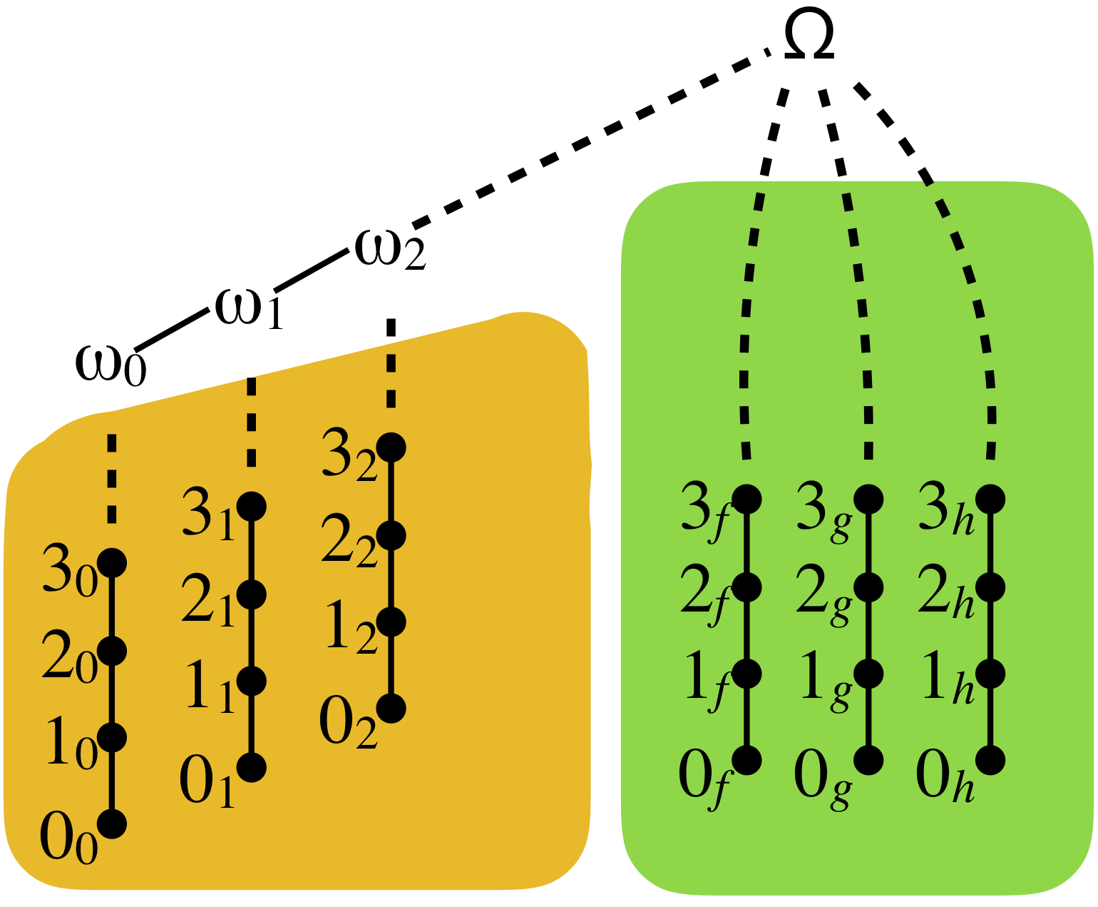
The gadget is obtained as follows. First, we take copies of N, with its usual ordering, one per natural number, and we put them side by side. This is the left part of the gadget, shown on an orange background. I will write mk for element number m in column number k.
On top of each orange column k, we add an element ωk, and we order them by ω1 ≤ ω2 ≤ … ≤ ωk ≤ … On top of that, we add a top element Ω.
Next, we build another set of copies of N (on the right part of the gadget, shown on a green background). Those copies are indexed by maps f : N → N, and they all have Ω as supremum. (Yes, there are uncountably many green columns.) I will write nf for the element number n in the green column f.
This gadget, per se, is not a complete lattice. It is a dcpo, though. One can check that it is sober, too. In particular, non-sobriety will not arise from the structure of the gadget.
Assembling the gadgets
Remember we wish to build a complete lattice L with infinitely many coatoms. To that end, we will assemble together infinitely many copies of the gadget, in such a way that their elements Ω are the desired coatoms. The point in having those funny orange and green parts in the gadgets is to organize the new ordering relations which we shall require between elements of different copies of the gadget.
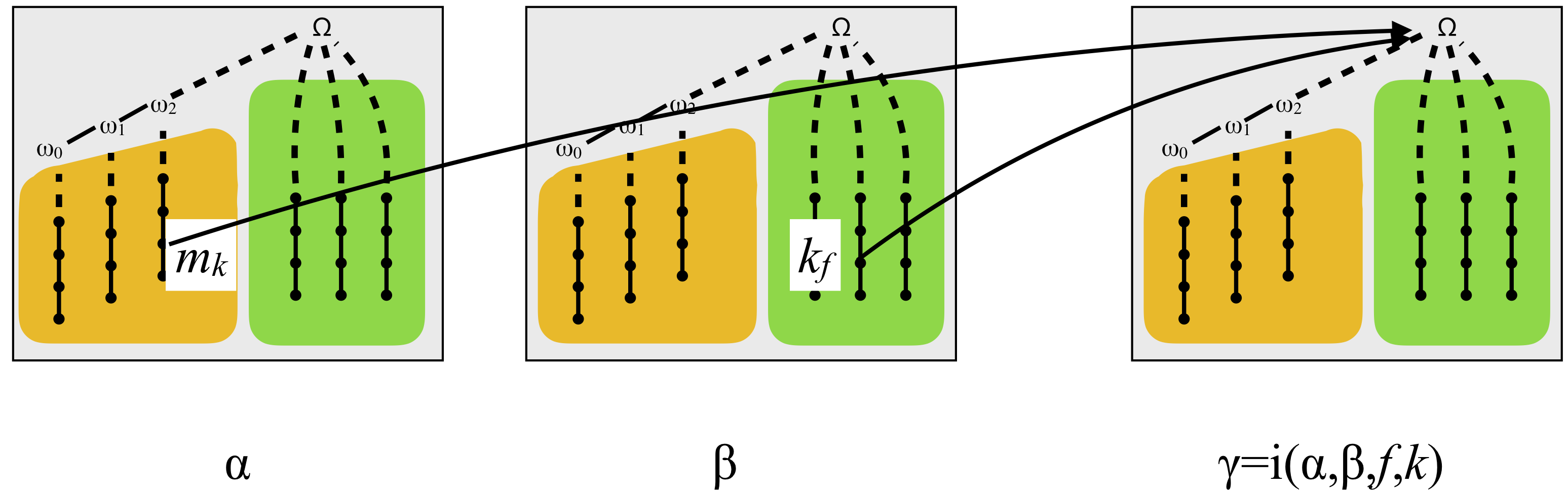
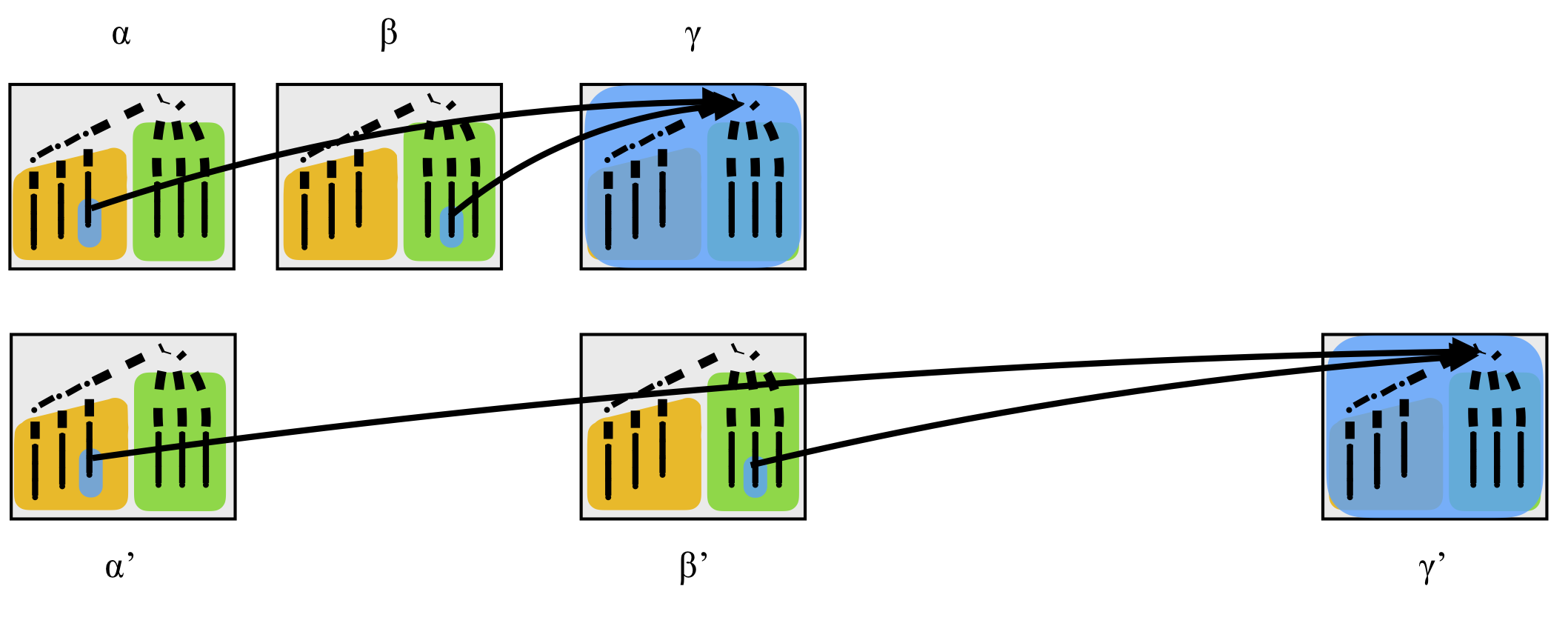
First, we put c many copies of Isbell’s gadget side by side, where c is the cardinality of R. Those copies will be indexed by positive real numbers α, β. (Isbell uses ordinal numbers < c, but I feel that using real numbers will be easier. It will certainly allow me to give a completely explicit definition of the map i below. This is the announced modification to Isbell’s construction, and that is entirely benign.)
We consider the elements of gadget number α and those of gadget number β (α≠β) as incomparable, except for the following new relations. Whenever α≠β:
- given any element mk from the orange part of gadget α,
- and any element kf from the green part of gadget β,
- with m=f(k) and n=k,
- we pick element Ω from gadget γ, for some γ>α,β that is uniquely determined as a function i(α, β, f, k) of α, β, f, k (and m=f(k) and n=k), and we declare that that element is above both mk and kf. See the picture below. This actually makes that element Ω from gadget γ the supremum of mk (from gadget α) and nf (from gadget β).
That will not be enough to build a lattice (yet). The main point of this construction is to ensure non-sobriety. The second point of this construction is that it is so sparse that embedding it into a complete lattice will be manageable.
For now, let us check non-sobriety. Build the poset P indicated above: take a disjoint union of gadgets indexed by positive real numbers α, β, add all the relations given in the picture, for all α, β, f, k, with α≠β, and where γ is computed as some function i(α, β, f, k) so that γ>α,β. (We will also want i to be injective, and therefore we will have to verify that such an injective function i exists. Let us postpone that for the moment.)
- The only non-trivial chains in P (i.e., those that are infinite) lie entirely inside one column (orange or green) of one gadget, or eventually form a chain among the elements ωk of that gadget: as in Johnstone space J, if you go up a column (or a chain of elements ωk) and then decide to leave it, you will instantly reach a topmost element Ω, and stop. From that it is easy to see that P is a dcpo.
- Now, let us consider any two open subsets U and V that meet P (i.e., that are non-empty). U meets gadget number α for some α, and V meets gadget number β for some β. Hence they contain the element Ω in these respective gadgets. If α=β then that element Ω is common to both gadgets, hence is in U ∩ V. Henceforth let us assume that α≠β.
- Since U is Scott-open and contains the element Ω of gadget α, it must contain the element ωk from that gadget for k large enough, say k≥k0. For each k≥k0, still by Scott-openness it must contain some element mk from the orange part of gadget α. That m will depend on k: for each k≥k0, we pick an m such that mk is in U. Let us write that m as f(k). That defines a function f : N → N, at least its values on all k≥k0; for the remaining values of k, we define f(k) arbitrarily.
- V contains the element Ω of gadget β. We look at column number f in the green part of that gadget, where f is the function we have just defined. By Scott-openness V must contain an element kf from the green part of gadget β, for k large enough.
- We pick k above k0, we let m=f(k), so that the element mk from the orange part of gadget α is in U. The construction of P is done so that element Ω from gadget γ, where γ=i(α, β, f, k), will be both in U and in V. In particular P meets U ∩ V.
- This shows that P is irreducible, and clearly it is not the downward closure of a point, so P is not sober.
P is not sober, but we already knew of a (simpler) dcpo that is non-sober [1]. The second purpose of the above construction is that P is so sparse, in a sense, that we can complete P and obtain a complete lattice L with very few additional elements (still uncountably many…), compared to P. There will be so few of them that all the essential properties of P will remain true in L.
Before I explain why, let me justify why the injective map i exists.
The map i
Isbell is very implicit about the existence of i, and I would like to give a concrete proof of its existence.
First, there is a bijection between N × N and N. My preferred one maps m, n to ⟨m,n⟩ defined as follows. Write m and n in binary, hence as infinite sequences of bits that are ultimately zero. (I will write those infinite sequences as usual, namely extending infinitely to the left.) Then interleave those two sequences of bits, and read the result in binary: this is ⟨m,n⟩. For example, ⟨…001011,…100111⟩=…010010011111, where I have underlined the bits coming from n to make the process easier to understand. It is pretty easy to see that ⟨m,n⟩≥m, n for all m, n.
Next, there is an injection from [0,1) × [0,1) into [0,1). There is even a bijection, but I won’t need that. To build that injection, take any two numbers α, β in [0,1), write them in binary as 0 comma followed by an infinite sequence of bits (which does not end in all ones—and those extend infinitely to the right), interleave the sequences of bits again, and read the result in binary, c(α, β).
It follows that there is an injection from (0,1] × (0,1] into (0,1]: this maps α, β in (0,1] to 1–c(1–α, 1–β). By suitable translations, we obtain injections cm,n from (m, m+1] × (n, n+1] into (⟨m,n⟩+1, ⟨m,n⟩+2], for all natural numbers m and n.
Let R+ be the set of positive real numbers (excluding zero). We can build an injection d of R+ × R+ into R+ as follows. For all α, β in R+, there are unique natural numbers m and n such that α is in (m, m+1] and β is in (n, n+1]. We let d(α, β)=cm,n(α, β). This is clearly an injection, and we have d(α, β) > ⟨m,n⟩+1, which is larger than or equal to m+1 ≥ α, and also to n+1 ≥ β. Hence d(α, β) > α, β for all α, β in R+.
Next, we fix an injection J from N → N to R+. Again, we could even require a bijection, but an injection is easy to give explicitly. For every f : N → N, we form the set A of all natural numbers ⟨m,f(m)⟩, and then we convert A into the real number 1+∑i ∈ A 2/3i for example.
We now define i(α, β, f, k) as d(α, d(β, d(J(f), k))). This is injective, and i(α, β, f, k) > α, β for all α, β in R+, as required.
Forming the final complete lattice
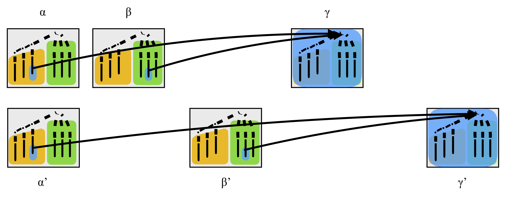
We take the dcpo P we have constructed by assembling uncountably many copies of Isbell’s gadget, with the extra relations shown in Figure 2: the element Ω from gadget γ=i(α, β, f, k) is above the element mk from the orange part of gadget α (with m=f(k)) and above the element kf from the green part of gadget β, for all α≠β.
Isbell has a very simple way of building a complete lattice L out of P: we just take all intersections of principal ideals ↓x, x in P, and we order those intersections by inclusion. This is a very simple construction, but it will take us some effort to understand its structure. If you think that is too hard, please skip to the next section, and I will give you another construction of a non-sober complete lattice based on P in a more direct way [5]. That other construction will be much more implicit, though, but it will also give us more.
L is automatically a complete lattice, because it has all infima, computed as intersections. This is because the elements of L were already defined as arbitrary intersections of certain sets.
Also, we can equate every element x of P with the element ↓x of L, so L is a complete lattice that contains P.
Suprema in L may appear to be hard to compute at first, until we realize that P was so sparse that L has very few additional elements (still uncountably many, but organized in a very simple way), compared to P. We will determine those extra elements explicitly.
First, as in every lattice, there is a top element ⊤, above all the elements Ω of each gadget, and there is a bottom element ⊥ below all elements of all gadgets. The top element ⊤ is the intersection of a family of 0 principal ideal. Let us look at the intersections of two principal ideals. We will see that some of them represent fresh elements, in L but not in P, and also that these are the only ones.
In order to determine what the intersections of two principal ideals of P are, we first classify the principal ideals ↓x of P. Let me classify them into five types (see Figure 3 below). Type I is the case where x=mk in gadget α. Type II is the case where x=ωk, still in gadget α. Type III is the case where x=kf, again in gadget α. The final two types are when x=Ω in some gadget γ: type IV is when γ is not in the range of i, and consists of just the whole of gadget γ, while type V is when γ=i(α, β, f, k), and consists of the whole gadget γ, plus ↓mk (with m=f(k)) and ↓kf in gadgets α and β respectively. Note that in the latter case, α, β, f, k are determined uniquely as a function of γ, because i is injective, and that α and β are both < γ and distinct. All those cases are represented below, as blue regions.
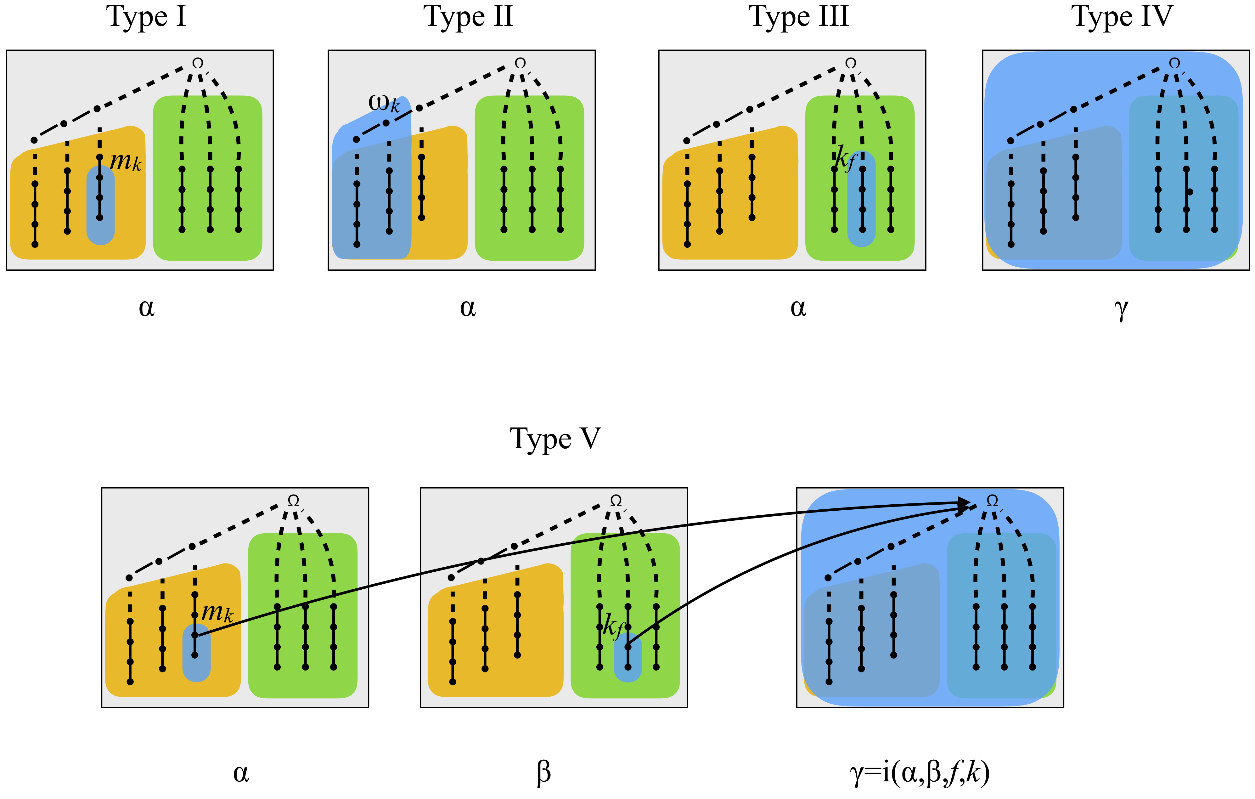
I have summarized all the subsets of P that we can get by intersecting two principal ideals in the following table. This reads as follows. Say you wish to know what kind of set we can get by intersecting a Type I and and Type IV ideal. The cell at coordinates “Type I” and “Type IV” in the following table says “I/∅”, and that means you will get either a Type I ideal or the empty set (the bottom element of L). I have not shown any cell below the diagonal: you can fill the remaining cells by symmetry.
| Type I | Type II | Type III | Type IV | Type V | |
| Type I | I/∅ | I/∅ | ∅ | I/∅ | I/∅ |
| Type II | II/∅ | ∅ | II/∅ | I/II/∅ | |
| Type III | III/∅ | III/∅ | III/∅ | ||
| Type IV | IV/∅ | I/III/IV/∅ | |||
| Type V | I/III/V/∅/I ∪ III |
The only interesting case is what happens when you intersect two Type V ideals. The corresponding cell says “I/III/V/∅/I ∪ III”, and that means that the intersection can be a Type I ideal, a Type III ideal, a type V ideal, the empty set… or the union of a Type I ideal and of a Type III ideal. In the latter case, those two principal ideals will be in different gadgets, the Type I part will be equal to ↓mk from the orange part of its gadget and the Type III part will be equal to ↓kf from the green part of its gadget—with m=f(k), which means that knowing the column numbers k and f completely determine mk and kf.
Let me check that explicitly. Imagine you intersect two Type V ideals, one involving gadgets α, β, and γ=i(α, β, f, k) (with γ>α, β and α≠β) and the other one involving gadgets α’, β’, and γ’=i(α’, β’, f‘, k‘) (with γ’>α’, β’ and α’≠β’). If γ=γ’, then since i is injective, the two ideals must be the same, and their intersection will therefore trivially have Type V. Let me assume γ≠γ’. There are many cases where the intersection will be empty, and the only cases where it is not are:
- when their α-gadgets intersect: α=α’ and k=k‘
- when their β-gadgets intersect: β=β’ and f=f’
- when α=γ’
- when β=γ’
plus all symmetric cases, where the unprimed and primed ideals are exchanged.
In case 1, we cannot have β=β’ and f=f’, otherwise γ would be equal to γ’. It may be that γ=β’, though, and then the intersection is one Type I ideal from gadget α, plus one Type III ideal from gadget β’:
It may also be that β=γ’. That is a symmetric case, with the same outcome.
Still in case 1, it may also be that β=β’ and f≠f’, in which case the intersection is just one Type I ideal from gadget α. The final subcases, where β≠β’, γ≠β’ or β≠γ’, gives the same kind of result, see the following picture.
In case 2 (β=β’ and f=f’), a similar reasoning shows that we obtain either one Type I ideal from gadget α, plus one Type III ideal from gadget β, or just one Type III ideal. And we obtain the same results in cases 3 and 4, which overlap with the previous cases partly.
The Type I ∪ III ideals themselves intersect with sets of Type I ∪ III, I, II, III, IV, or V as follows.
| Type I ∪ III | Type I | Type II | Type III | Type IV | Type V | |
| Type I ∪ III | I/III/I ∪ III/∅ | I/∅ | I/∅ | III/∅ | I/III/∅ | I/III/∅ |
This implies that we know what all the finite intersections of principal ideals of P are: apart from the intersection of zero ideal (the top element ⊤) and the empty set (the bottom element ⊥), we have the Type I through Type V ideals (already represented as elements of P), plus the sets of Type I ∪ III, which one can represent as fresh infima of certain pairs of elements Ω from different gadgets.
Arbitrary intersections of principal ideals of P can be written as filtered intersections of finite intersections. We know all the finite intersections, and it is pretty easy to see that those finite intersections are well-founded: you cannot form infinite decreasing chains. (If a Type IV or Type V ideal contains a finite intersection of ideals strictly, then it must be of another type. If a Type I ∪ III set contains a finite intersection of ideals strictly, it must be empty or of Type I or of Type III. If a Type II ideal contains a finite intersection of ideals strictly, then it must be empty of of Type I. Then Type I ideals, as well as Type III ideals, are clearly well-founded.)
It follows that we have found all the elements of L: they are the elements of P, plus a top element ⊤, plus a bottom element ⊥, plus fresh infima of certains pairs of elements Ω from different gadgets, represent as Type I ∪ III sets. That is it.
Non-sobriety
Now that we have formed the final complete lattice L, the argument that we had used to show that P is not sober applies almost verbatim to show that L is not sober either. Let C be the whole of L except the top element ⊤.
- The only non-trivial chains in L (i.e., those that are infinite) lie entirely inside one column (orange or green) of one gadget, or eventually form a chain among the elements ωk of that gadget. In particular they are entirely in P, so their supremum is in C. That shows that C is Scott-closed.
- Now, we consider any two open subsets U and V that meet C. U meets gadget number α for some α, and V meets gadget number β for some β. Hence they contain the element Ω in these respective gadgets. If α=β then that element Ω is common to both gadgets, hence is in U ∩ V. Henceforth let us assume that α≠β.
- Since U is Scott-open and contains the element Ω of gadget α, it must contain the element ωk from that gadget for k large enough, say k≥k0. For each k≥k0, still by Scott-openness it must contain some element mk from the orange part of gadget α. That m will depend on k: for each k≥k0, we pick an m such that mk is in U. Let us write that m as f(k). That defines a function f : N → N, at least its values on all k≥k0; for the remaining values of k, we define f(k) arbitrarily.
- V contains the element Ω of gadget β. We look at column number f in the green part of that gadget, where f is the function we have just defined. By Scott-openness V must contain an element kf from the green part of gadget β, for k large enough.
- We pick k above k0, we let m=f(k), so that the element mk from the orange part of gadget α is in U. The construction of P is done so that element Ω from gadget γ, where γ=i(α, β, f, k), will be both in U and in V. In particular P, hence C, meets U ∩ V.
- This shows that C is irreducible, and clearly it is not the downward closure of a point, so L is not sober.
A non-sober frame
Isbell’s non-sober complete lattice L is not distributive. Take any element a=mk from the orange part of gadget α (for any α), any element b=kf from the orange part of gadget β (for any β≠α), with m=f(k), and any element c from the orange part of gadget γ=i(α, β, f, k). Then a ∨ b is the element Ω of gadget γ, so (a ∨ b) ∧ c = c, while (a ∧ c) ∨ (b ∧ c) = ⊥ ∨ ⊥ = ⊥.
Is there any non-sober distributive complete lattice? This was answered recently by Xu, Xi and Zhao [5]. They show that there is even a non-sober frame. (It is even spatial, but I will not explore this here.)
That frame is Q(L), the poset of non-empty compact saturated subsets of L with reverse inclusion as ordering. Since L is a complete lattice, it is well-filtered [3], and therefore coherent [4]. It is also compact, because it has a least element. It follows that every intersection of elements of Q(L), which can be written as a filtered intersection of finite intersections, is again an element of Q(L). It is clear that any finite union of elements of Q(L) is again in Q(L). Moreover, intersections distribute over binary unions: Q(L) is a frame. It only remains to show that Q(L) is not sober.
If you have skipped the previous section on the construction of L, we can alternatively consider a non-sober frame as Q0(P⊥), the poset of compact saturated subsets (including the empty one) of P⊥, where P⊥ is P with an extra bottom element ⊥. P⊥ is not a lattice, but it is bounded-complete: every family that has an upper bound has a least upper bound. Indeed, any family that has an upper bound must have some element Ω of some gadget γ as upper bound, and must therefore be included in a Type IV or in a Type V ideal (see previous section); the result then follows by inspection of the different cases that can happen. The Lawson-Xi result [3] does not just say that every complete lattice is well-filtered, but also that all bounded-complete lattices are well-filtered. In a bounded-complete lattice, the intersection ↑x ∩ ↑y of two principal filters is empty or a principal filter, and compact in any case. Therefore the Jia-Jung-Li result [4] again applies: P⊥ is coherent. Since it has a bottom element, it is itself compact. By a similar argument as in the previous paragraph, this implies that Q0(P⊥) is a frame. We will show that it is not sober.
Given any topological space X, we have two topologies on Q0(X) (resp., Q(X)): the Scott topology of reverse inclusion, and the upper Vietoris topology. The latter has subbasic open sets ☐U, U open in X, where ☐U is the set of (non-empty) compact saturated sets included in U. When X is well-filtered, the directed suprema of compact saturated sets are computed as their intersection, and ☐U is Scott-open (Proposition 8.3.25 in the book). Also, if X is a well-filtered dcpo in its Scott topology, then the map η : X → Q0(X) (resp., Q(X)) is continuous, whichever of the two topologies we put on the target space. This is easy for the upper Vietoris topology, because η-1(☐U)=U. For the Scott topology, we realize that for every directed family (xi)i ∈ I in X, η(supi ∈ I xi) = ↑supi ∈ I xi = ∩i ∈ I ↑xi = supi ∈ I η(xi).
The key is the following result of Xu, Xi and Zhao [5, Theorem 1]:
Proposition. Let X be a well-filtered dcpo in its Scott topology. If Q0(X) (resp., Q(X)) is sober in its Scott topology, then X is sober.
Note: Xu, Xi, and Zhao prove that, more generally, for all T0 topological spaces X such that η is continuous when the target space is regarded with the Scott topology, and such that the upper Vietoris topology is coarser than the Scott topology on Q0(X) (resp., Q(X)).
Proof. Let C be any irreducible closed subset of X. Then the closure of the image of C by η, cl(η[C]), is irreducible closed in Q0(X) (resp., Q(X)), because that is Sη(C) (we apply the sobrification functor S to the continuous map η). Note that closure is taken in Q0(X) (resp., Q(X)). Since Q0(X) (resp., Q(X)) is sober by assumption, cl(η[C]) is the downward closure of some compact saturated set Q0 (resp., non-empty). Remembering that the ordering on compact saturated sets is reverse inclusion, cl(η[C]) is then the set of all compact saturated sets that contain Q0.
We claim that: (1) for every x in C, for every y in Q0, x≤y. Indeed, for every x in C, η(x)=↑x belongs to η[C] hence to cl(η[C]), so it contains Q0.
Next: (2) Q0 is supercompact, namely for every open cover (Ui)i ∈ I of Q0, Q0 is included in some Ui. Let us prove this. Q0 is in cl(η[C]) and in the upper Vietoris open set ☐(∪i ∈ I Ui). Since the upper Vietoris topology is coarser than the Scott topology (the one we take on sets of compact saturated sets), ☐(∪i ∈ I Ui) is (Scott-)open. It intersects cl(η[C]) (at Q0), hence it also intersects η[C]. This means that there is a point x in C such that ↑x is in ☐(∪i ∈ I Ui). Then x is in ∪i ∈ I Ui, hence in some Ui. By (1) above, x is below every element of Q0. This implies that Q0 is included in Ui.
It follows: (3) Q0 is of the form ↑x0 for some point x0. This is general fact: every supercompact saturated set (in any topological space) is the upward closure of some point. This can be found as Fact 2.2 in [6], another very interesting and very useful paper. The proof is pretty simple. We take the family (Ui)i ∈ I consisting of the complements of the sets ↓x, x in Q0. No Ui can contain Q0, by definition. By supercompactness, Q0 cannot be included in ∪i ∈ I Ui, hence Q0 must intersect its complement, say at x0. Then x0 is in Q0, and in all the sets ↓x, x in Q0. That means that x0 is the least element of Q0, as desired.
To recapitulate, cl(η[C]) is the family of compact saturated sets that contain Q0=↑x0=η(x0). Recall that by (1) x0 is above every element of C. We wish to show that C=↓x0, and that will prove the Proposition. For that, it only remains to show that x0 is in C. Imagine it is not. Then it is in the complement U of C, which is open in X. Then Q0=↑x0 is in ☐U, so ☐U intersects cl(η[C]). Since ☐U is upper Vietoris open hence (Scott-)open, ☐U also intersects η[C]. Hence there is a point x in C such that ↑x is in ☐U. Then x is in C, and also in U, contradiction. ☐
The Proposition allows us to conclude. P⊥ is a well-filtered dcpo, and is not sober (way back in this post, we have proved that P is not sober, and the same argument works for P⊥). Hence Q0(P⊥) is not sober. Finally, we recall that Q0(P⊥) is a frame.
Xu, Xi and Zhao use the same argument to show that Q(L) is a non-sober frame. Their paper [5] is a recommended read. They also show that a topological space X is well-filtered if and only if Q(X) with the upper Vietoris topology is well-filtered. That is a very nifty result, whose proof is very non trivial (and uses the Axiom of Choice at every step, as Zhenchao Lyu expressed it).
- Peter T. Johnstone. Scott is not always sober. Lecture Notes in Mathematics 871, Springer-Verlag, Berlin and New York, pages 282-283, 1981.
- John Isbell. Completion of a construction of Johnstone. Proceedings of the American Mathematical Society 85(3), pages 333-334, July 1982.
- Jimmie Lawson and Xiaoyong Xi. On well-filtered spaces and ordered sets. Topology and its Applications 228(1), September 2017, pages 139-144.
- Xiaodong Jia, Achim Jung, and Qingguo Li. A note on the coherence of dcpos. Topology and its Applications, Volume 209, 15 August 2016, Pages 235–238.
- Xiaoquan Xu, Xiaoyong Xi, and Dongsheng Zhao. A complete Heyting algebra whose Scott space is non-sober. arXiv:1903.00615, March 2019.
- Reinhold Heckmann and Klaus Keimel. Quasicontinuous domains and the Smyth powerdomain, Electronic Notes in Theoretical Computer Science 298(2013), pp. 215–232.

— Jean Goubault-Larrecq (April 21st, 2019)